· Michele Mazzucco · Post · 15 min read
When hybrid queues beat hiring during seasonal spikes — A 3‑step ROI playbook
We present an executive playbook comparing a combination of hybrid physical and digital queueing to temporary staffing, with a compact ROI framework and a hypothetical case study decision-makers can use.

Peak demand forces decision makers to make a choice that looks binary but isn’t: quick temporary hires or investing in a hybrid physical plus digital queue?
Both have real costs and trade-offs. The goal of this playbook is to provide a compact ROI model and a worked example so you can decide—quickly and with confidence—whether hires or a hybrid queue deliver the better return for your business.
Table of contents
- A concise ROI approach for leaders
- Compact hypothetical case study
- Sensitivity snapshot
- Payback and amortisation
- Three-year comparison
- Social multiplier
- Executive takeaway
- Further reading
A concise ROI approach for leaders
When evaluating options, we focus on three things: money recovered (revenue and margin), speed-to-value (how quickly the option reduces abandonment), and long-term scalability (i.e., does the solution amortize across seasons and locations?).
While temporary hires excel at speed, hybrid solutions are more likely to win on scalability and customer experience. This article shows you how to compare them using three simple steps:
- Baseline: capture a single peak‑day snapshot. Record throughput (
T0), abandonment (A0), revenue per customer (R), peak hours (H) and peak days (D). - Translate: describe each option in terms of the incremental customers it serves and the total cost to deliver them (for hires, the seasonal staffing bill; for hybrid, the one‑off implementation plus recurring operating costs). Convert that to recovered gross by multiplying customers,
RandD, then apply a conservative margin to arrive at recovered margin. - Compare on the same timeline: amortise hybrid one‑offs across seasons or sites and run a short sensitivity sweep (pessimistic, likely, optimistic).
Compact hypothetical case study
In this article we make the following assumptions:
- Peak days: 26 per season. We assume shops remain closed on Sundays (≈6 days/week)
- Peak hours/day: 10
- Baseline peak customers/day: 1,200 (120/hr)
- Baseline abandonment: 8%, which corresponds to 96 lost customers per day
- Average revenue per served customer (
R): €25 - Temp hire cost: €30/hr
- Hybrid one-time cost: €30,000
- Hybrid monthly ops (sensitivity): €200 / €500 / €1,000 per site (we use these bands in the sensitivity examples)
- Hybrid likely impact: abandonment reduced to 2% (recover 72 customers/day); throughput uplift 15% (test uplift caps: 5% / 15% / 25% in sensitivity rows)
Use this example as a template and replace the above numbers with your own, if needed.
📌 Note on temp hire rates
Hire snapshot
One extra temporary hire (approximately 12 customers per hour) covers the worked peak. The seasonal staffing cost in our example is one hire × €30 per hour × 10 hours × 26 days, which equals €7,800. Temporary staff are useful fast fixes, but they rarely eliminate abandonment entirely.
Targets (symmetric with hybrid):
- Likely (both hires and hybrid): if abandonment is reduced to 2%, the seasonal recovered customers would be 1,872. That equals a gross recovered revenue of €46,800; applying a 30% margin gives €14,040 recovered margin and approximately €6,240 net after staffing costs.
- Optimistic: if abandonment can be reduced to 1%, the seasonal recovered customers would be 2,184. That equals a gross recovered revenue of €54,600; applying a 30% margin gives €16,380 recovered margin and approximately €8,580 net after staffing costs.
Use the symmetric likely/optimistic framing when you compare hires to hybrid; treat hybrid’s throughput uplift as an additive effect (separate from abandonment reduction) so you can see capacity gains independently.
Hybrid snapshot
Assume a lean pilot with a one‑off cost of €30,000 and ongoing ops that vary by implementation — we model a sensitivity band of €200 / €500 / €1,000 per month per site. With the likely impact in our example—abandonment reduced to 2% and throughput uplift of 15%—the hybrid recovers 72 customers per day (abandonment) plus the throughput uplift described below. Over 26 peak days the abandonment-only component equals 1,872 recovered customers; applying the combined uplift materially increases recovered customers (see worked example). In a single‑site, single‑season comparison hires can still look better; the hybrid option becomes compelling when you spread the one‑off cost across multiple sites or seasons and when you value a more consistent customer experience.
Figure 1 shows the annual net seasonal benefit after amortisation and recurring ops, for 1, 3 and 5 sites. Use it to compare the total cash advantage of a hybrid rollout as you scale: if your target site count lands the bar above zero in the likely case, the hybrid option delivers a positive recurring return and is worth a pilot.
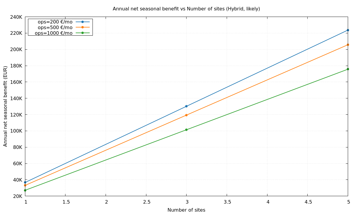
Note that the worked example includes two effects: (A) abandonment recovery (72 customers/day) and (B) a throughput uplift of 15%.
We treat the combined effect (abandonment + throughput) as the “likely” case and use it in the main narrative because it reflects the operational uplift we typically observe in pilots. A conservative, abandonment‑only view is kept in a collapsible box below for finance to stress‑test assumptions.
For clarity — combined effect example (baseline R = €25):
- Abandonment recovered: 72/day, or 72 × 26 = 1,872/season
- Throughput uplift (15% of baseline 1,200/day): 180/day, or 180 × 26 = 4,680/season
- Combined recovered customers: 1,872 + 4,680 = 6,552/season
- Combined recovered gross: 6,552 × €25 = €163,800
- Recovered margin (30%): €49,140/season
Interpretation: using the full hybrid effect (abandonment + throughput) changes the recovered margin from €14,040/season (conservative) to €49,140/season (likely) — a material difference that flips the long-term economics in most amortisation scenarios. This conservative view counts only abandonment recovery (72/day → 1,872/season) and ignores throughput uplift. It is useful for stress‑testing upside assumptions, but it understates the operational benefits we typically observe in pilots.Conservative baseline — abandonment-only
Sensitivity snapshot
Below are two short tables showing net seasonal benefit under sensible variations. All numbers assume recovered margin equals 30% of recovered gross. Net seasonal benefit is recovered margin minus the seasonal cost (staff cost for temporary hires or the amortised one‑off for the hybrid).
Temp hire scenarios (one extra temp for peak days)
| 💶 Hourly rate | 📆 Seasonal staffing cost (10h × 26d) | 📊 Recovered margin (30% of recovered gross) | 🔍 Net seasonal benefit |
|---|---|---|---|
| €25/hr | €6,500 | €18,720 | €12,220 |
| €30/hr | €7,800 | €18,720 | €10,920 |
| €35/hr | €9,100 | €18,720 | €9,620 |
Realistic hire targets (reduced abandonment to 1% or 2%)
| 🎯 Target abandonment | 📈 Seasonal recovered gross | 📊 Recovered margin (30% of recovered gross) | 👷 Staffing cost | 🔍 Net seasonal benefit |
|---|---|---|---|---|
| 1% | €54,600 | €16,380 | €7,800 | €8,580 |
| 2% | €46,800 | €14,040 | €7,800 | €6,240 |
Hybrid amortisation (recovered margin €14,040)
| 🏬 Amortisation across | 📈 Amortised one‑off per site | 📊 Recovered margin (30% of recovered gross) | 🔍 Net seasonal benefit |
|---|---|---|---|
| 1 site | €30,000 | €14,040 | −€15,960 |
| 3 sites | €10,000 | €14,040 | €4,040 |
| 5 sites | €6,000 | €14,040 | €8,040 |
The above tables make the trade-off explicit: temporary hires deliver a positive short‑term net benefit across typical rate bands; hybrid can be negative in a single‑site comparison but quickly becomes attractive when costs are spread across multiple locations or seasons.
The heatmap in Figure 2 shows profitability across two inputs: monthly ops cost (horizontal) and site count (vertical). Colours indicate annual net (green = profitable, red = loss).
Next, we show two views: the “Likely” heatmap (combined abandonment and throughput uplift) and a “Conservative” heatmap (abandonment‑only). Compare them to see where upside assumptions matter.
Under our combined uplift assumptions the tested configurations are profitable (yellow and green), see Figure 2. This reflects the operational uplift we typically observe in pilots; it shows the potential upside when throughput and abandonment recovery combine.
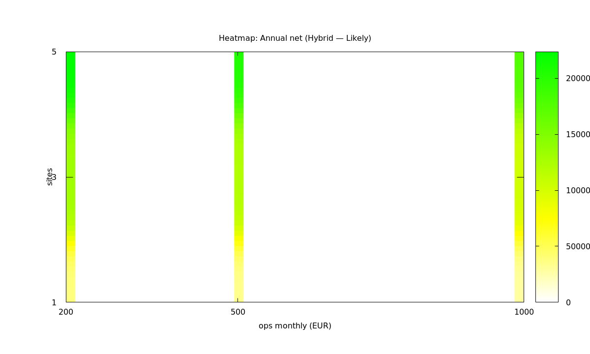
Figure 2 - Heatmap (Likely): annual net by ops/month and sites. Heatmap: red = loss, white = break‑even, green = gain.
On the other hand, Figure 3 shows that under conservative (abandonment‑only) assumptions small/expensive deployments can lose money (red). Use this view to identify risk areas where you should pilot or negotiate lower ops costs before scaling.
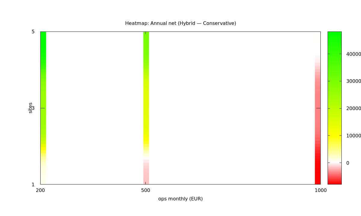
Figure 3 - Heatmap (Conservative): annual net by ops/month and sites. Heatmap: red = loss, white = break‑even, green = gain.
🚨 Important: the two heatmaps are a sensitivity pair
Takeway: if your expected ops and uplift match the Likely assumptions, the hybrid is broadly profitable; if you must assume the Conservative case, only roll out where the Conservative heatmap is green (or start with multi‑site pilots).
Payback and amortisation
You may reasonably ask how many seasons (or years) it takes to recover the hybrid investment. In our worked hybrid scenario the recovered margin is €14,040 per season. To calculate seasons-to-payback, divide the amortised one‑off cost per site by the recovered margin.
Payback (seasons) for the worked examples:
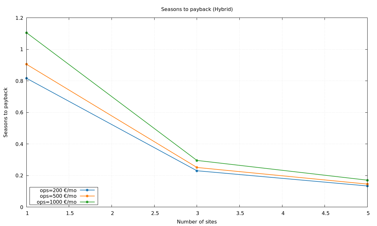
The seasons‑to‑payback values shown in the chart below are calculated from the annual net seasonal benefit (that is, recovered margin minus the annualised portion of the one‑off and any recurring ops). In other words, the plot answers: “How many seasons of net cashflow (after amortisation and ops) are required to recoup the €30k investment?” — this is a cashflow‑aware definition and is what we use for rollout decisions.
Example (Likely combined uplift, representative ops = €500/mo):
- One site: annual net ≈ €33,140, resulting in ≈ 0.9 seasons‑to‑payback (30,000 / 33,140).
- Three sites: annual net ≈ €119,420, resulting in ≈ 0.25 seasons‑to‑payback (30,000 / 119,420).
- Five sites: annual net ≈ €205,700, resulting in ≈ 0.15 seasons‑to‑payback (30,000 / 205,700).
For readers who prefer the simpler heuristic used earlier (ignore recurring ops), dividing the full one‑off by the recovered margin per season (30,000 / 14,040) gives ≈ 2.1 seasons — this ‘recovered‑margin only’ view is a quick rule‑of‑thumb but understates time‑to‑payback when ops and amortisation are material. The chart displays the stricter, cashflow‑aware payback values used for decision‑making.
📌 Note
You can shorten the payback time by:
- Piloting aggressively with a lean, software‑first approach to reduce one‑off costs.
- Leasing hardware or negotiating vendor trial discounts.
- Prioritising highest‑performing locations first to maximise recovered margin per site.
- Increasing retention and LTV (loyalty programs, follow‑up offers) to increase recovered margin per customer.
Use these calculations in the internal workshop to estimate realistic time‑to‑payback for your rollout strategy.
Figure 4 reports seasons‑to‑payback using annual net (recovered margin minus amortisation and ops). Values smaller than 1 mean the investment pays back inside one season; large or negative values indicate payback is slow or impossible under the tested assumptions.
When hiring scales: temporary capacity by recovered customers/day
Temporary hires are finite-capacity resources. Use this quick mapping to see when a single temp is no longer enough and you must add another hire (approximate, based on the worked example assumptions):
| Recovered customers/day | Temps needed (≈120 customers/day per temp) |
|---|---|
| 0–120 | 1 |
| 121–240 | 2 |
| 241–360 | 3 |
| 361–480 | 4 |
Example: if the hybrid (including throughput uplift) recovers 240 customers/day, that is roughly 2 temporary hires worth of capacity — doubling the seasonal staff cost if you chose hires instead of hybrid.
Three-year comparison
Below are two compact views of the worked example across a 3-year window; they illustrate the amortisation effects.
Note: the article’s primary narrative and the figures above use the combined (abandonment + throughput) numbers as the likely case; the tables below show optimistic vs conservative amortisation views to stress-test outcomes (the “Conservative” rows use the abandonment-only margin — see the conservative baseline above).
Assumptions repeated from the worked example:
- Recovered margin (hire scenario — likely, 2% abandonment): €14,040 per season — Recovered margin (hybrid per site — conservative, abandonment-only 2%): €14,040 per season — Likely combined hybrid recovered margin (abandonment 2% + 15% throughput, R=€25): €49,140 per season
- Temp seasonal staff cost (one hire): €7,800 per season
- Hybrid one-off: €30,000 total
- Hybrid monthly ops per site (sensitivity): €200 / €500 / €1,000 per month (i.e., €2,400 / €6,000 / €12,000 per year)
Optimistic view — exclude recurring ops (shows pure amortisation effect)
| Scenario | Annual recovered margin | Annual amortisation (one-off / 3 years) | Annual cost | Annual net | 3‑year cumulative net |
|---|---|---|---|---|---|
| Hire (one temp) | €18,720 | €0 | €7,800 (staff) | €10,920 | €32,760 |
| Hybrid — 1 site | €14,040 | €10,000 | €10,000 | €4,040 | €12,120 |
| Hybrid — 3 sites (one‑off split) | €42,120 | €10,000 | €10,000 | €32,120 | €96,360 |
Conservative view — include recurring ops (our example uses €500/mo per site; run sensitivity tests at €200 / €500 / €1,000, if needed).
| Scenario | Annual recovered margin | Annual amortisation (one-off / 3 years) | Annual recurring ops | Annual cost (amort + ops) | Annual net | 3‑year cumulative net |
|---|---|---|---|---|---|---|
| Hire (one temp) | €18,720 | N/A | N/A | €7,800 (staff) | €10,920 | €32,760 |
| Hybrid — 1 site | €14,040 | €10,000 | €6,000 | €16,000 | −€1,960 | −€5,880 |
| Hybrid — 3 sites (total) | €42,120 | €10,000 | €18,000 | €28,000 | €14,120 | €42,360 |
Notes:
- “Optimistic” assumes operations costs are negligible or already budgeted; it isolates the pure effect of amortising the one‑off over multiple years/sites. — “Conservative” adds the recurring ops line (€500/month per site in this example) which materially affects annual net and multi‑year cumulative results.
- You may use the optimistic for strategic investment comparisons, and the conservative view for tight-budget reality checks.
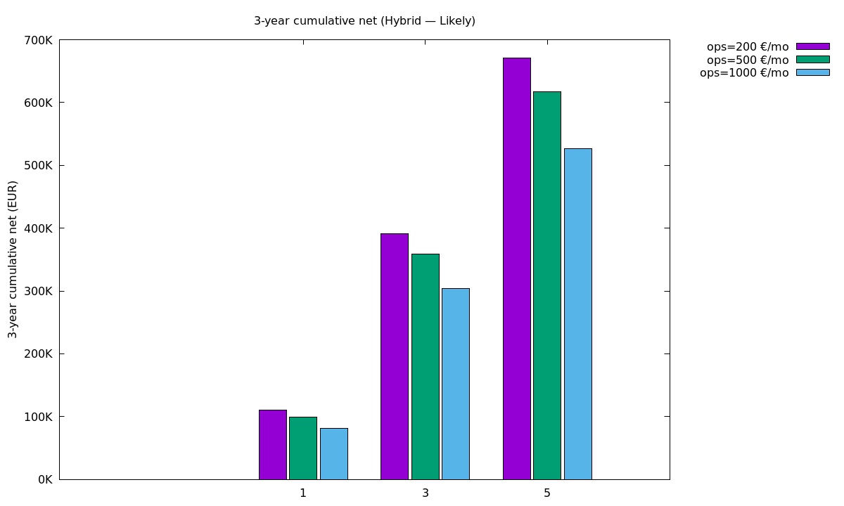
Figure 5 below sums the annual net over three years so you can see the multi‑year payoff after amortisation. Taller positive bars mean a larger cumulative return over 3 years; negative bars mean the investment hasn’t paid off in that window. Use this to pick your target horizon: if you need returns inside 3 years, prefer configurations with positive 3‑year bars.
Social multiplier
Word‑of‑mouth (WOM) matters, but in conservative models its direct effect is modest. Using a sharing rate of 10% and a conversion rate of 5% in our worked example adds roughly €1,000 of recovered margin for a single season. If referred customers have a meaningful lifetime value, multiply their single‑visit revenue by an LTV factor to reflect repeat visits; that can materially increase the WOM impact.
Suggestion: include a conservative plus/minus WOM row in your sensitivity tables rather than relying on referrals to change the core decision.
Including lifetime value (LTV)
To make the model more realistic for decision-making, it’s useful to value referred customers using a lifetime value (LTV) rather than single-visit revenue. A conservative default is LTV = 3 × R (three visits or equivalent future value). Using that assumption changes the worked numbers as follows (same sharers/new-customer counts as above):
- Default LTV = three times R, so 3 × €25 = €75.
- Hire: with 156 new customers and an LTV of €75, gross LTV is €11,700; at a 30% margin this implies about €3,510.
- Hybrid: with roughly 151 new customers and an LTV of €75, gross LTV is approximately €11,325; at a 30% margin this implies about €3,398.
Interpretation: applying a modest LTV multiplier increases the positive WOM uplift materially (from ~€1.1k margin to ~€3.4k margin in our example), so where referred customers are likely to return or have higher lifetime value the hybrid option’s indirect benefits become more meaningful. As always, allow execs to swap the LTV multiplier in the workshop to reflect their business model and retention expectations.
Compounding WOM (generation effects)
Referrals can compound: customers you acquire may in turn share and recruit others. A compact way to model this is geometric growth where the generation multiplier g = p_share × p_conv. Total cumulative new customers from one initial wave is roughly N_initial × (1 / (1 − g)) when g < 1.
Worked example (using a sharing rate of 10% and a conversion rate of 5%)
- The generation multiplier
gis the product of the sharing rate and the conversion rate. With a 10% sharing rate and a 5% conversion rate,gequals 0.005. - The cumulative multiplier is 1 divided by
(1 - g). Withg = 0.005that gives about 1.005, which corresponds to a 0.5% uplift on the initial acquired customers. - For the hire case: an initial 156 new customers becomes roughly 156.8 after compounding (an increase of about 0.8 customers).
- For the hybrid case: an initial 151 new customers becomes roughly 151.8 after compounding (also about +0.8 customers).
Interpretation: at conservative sharing and conversion rates compounding only adds a rounding effect. It becomes meaningful when either share or conversion rates are much higher (for example, when the product p_share × p_conv ≥ 0.02).
📌 Why €30k for the hybrid one‑off?
Executive takeaway
From the above exercise, we can summarize three short learnings:
- Small, single-site peaks: go for temporary hires. They are a fast and low-commitment solution, and usually offer the best short-term net benefit.
- Multi-site or repeatable peaks: choose hybrid queues. While they have a higher upfront cost, they provide better scalability, fewer escalations and superior CX once amortised.
- Always run the numbers on the same timeline and stress-test pessimistic/likely/optimistic scenarios rather than trusting point estimates.
Caveat: your mileage will vary — swap in your actual temp rates, vendor quotes and uplift assumptions in the workshop model. Use a lean pilot to validate operational uplift before a larger rollout.
Executive 30–60 minute checklist:
- Bring baseline (
T0,A0,R,H,D) for 1–3 sites. - Run the model: Hire (seasonal staff cost) vs Hybrid (amortised one‑off + ops) across conservative/likely/optimistic rows (include ops = €500/mo in the conservative row).
- Prioritise a pilot site or small cluster: choose the option that scores best on Speed-to-value, Net seasonal benefit and Scalability.
Further reading
Below are four short, related reads that provide deeper background and practical how‑tos you can consult after this playbook:
- The myth of more staff: why throwing people at long queues doesn’t work
- Why long wait times are costing your business more than you think
- No-wait secrets: when physical lines beat virtual—and vice versa
- From frustration to 5 stars: a modern guide to hotel and hospitality queues
📬 Get weekly queue insights
Not ready to talk? Stay in the loop with our weekly newsletter — The Queue Report, covering intelligent queue management, digital flow, and operational optimization.