· Michele Mazzucco · 17 min read
Virtual queues from scratch, Part 4: implementing admission control
Part 4 of our hands‑on series: harden your virtual queue for production with adaptive admission control, edge protection, and robust backend isolation—ensuring stability under any load.

Missed Part 3? Catch up here.
In our “Virtual Queues from Scratch” series, we have steadily progressed from abstract concepts to a functional component. Part 1 laid down the architectural blueprint and core principles of virtual queues. Part 2 brought the design to life by implementing our lean Python ASGI Lobby Service, leveraging Redis for robust state management. In Part 3, we tackled ticket flow, liveness detection, and the use of Python coroutines for realistic backend simulation.
With these foundations in place, this fourth installment is all about admission control and backend protection. Here, we address the challenge of keeping our system stable under any load by implementing dynamic, adaptive safeguards that prevent the queue from growing unbound and protect our backend from catastrophic overload. We focus on:
- Admission control: Strategic, load-aware decisions about when to accept or reject new requests, ensuring predictable performance and robust overload protection.
- Edge protection and horizontal scaling: Leveraging OpenResty and Redis to enforce admission logic consistently across all backend instances.
This article is your guide to building a virtual queue that remains resilient, responsive, and production-ready—even under the most demanding conditions.
Table of contents
Part E - Backend protection
Recent DoS attacks remind us that every system needs protection, even a virtual lobby.
The CL.THROTTLE command (originally from redis-cell) is a rate-limiter primitive, based on the GCRA algorithm — a smarter variant of leaky bucket:
- Maintains a sliding window (not fixed bucket refill intervals)
- Efficiently limits the rate per user / token / key
- Lightweight and atomic: doesn’t require background jobs or cleanup
It is useful to gate requests per API key or IP address, ensuring that each key can’t exceed N ops per second (or minute).
As described in this SeatGeek presentation, depending on the use case, you may want your queue to be stateless, stateful, or select users randomly. Our use case requires a stateful virtual lobby. This allows us to serializes requests beyond capacity, maintaining the order at which requests join our queue:
- At most
ctokens are processed concurrently - Excess requests are parked and informed of their position
- As we highlighted in our previous article, virtual queues are not just a fancy load balancer —they manage expectations. We do so by providing a feedback that includes queue size, ETA and a confidence level.
The estimated residual waiting time is based on user’s current position in the queue, runtime statistics and queueing approximations, while the confidence level can be used to enhance the users’ experience: as an example, instead of saying “residual time: 10 minutes”, you could provide a range “between 9 and 11 minutes” or a confidence band “we are 95% sure you will be served in 10 minutes”.
1. Admission control with hard thresholds (naive approach)
We have seen how Dragonfly’s built-in CL.THROTTLE command is excellent for per-user rate limiting, but not for protecting a global virtual queue. In our system, we want to accept requests but serialize their execution — something that CL.THROTTLE intentionally avoids (it rejects excess traffic).
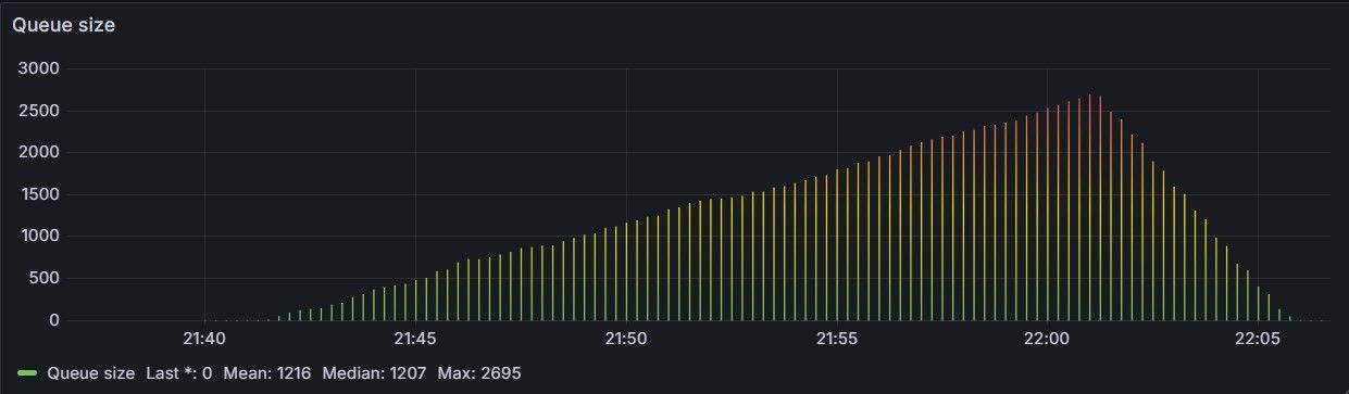
Still, it may be used as a pre-lobby filter to prevent bursts or abuse from overwhelming the queue: as an example, with 10 workers and a mean service time of one second, you can drain at most 10 req/sec on average. Accepting 1,000 req/sec means Redis will fill up with parked tokens at 990 req/sec — until memory runs out, capacity increases, or demand decreases — whatever happens first. An example of a queue growing unbound is shown in Figure 1.
The simplest admission control policy is a hard threshold: estimate the expected waiting time for a new request, and accept it only if the wait is below a fixed limit T. In formula:
accept if est_wait < T, else reject
where
est_wait = queue_size / (c * μ)
Here, queue_size is the number of jobs in the queue, c is the number of servers (i.e., our coroutines), and μ is the throughput of each server. If the estimated wait exceeds T, the request is rejected (e.g., with HTTP 429). This keeps the queue bounded and prevents runaway overload.
Please note that the pre-filtering does not require absolute accuracy, as this mechanism kicks-in only when the queue size grows large (how large is a tunable parameter). As this occurs only during traffic bursts (or if capacity drops), the queue build-up will not resolve instantly.
💡 Queueing theory note: depending on how we tune the admission control parameter, this part of the system will behave either like an M/M/n queue (admit all traffic) or an M/M/n/K queue (at most K jobs can be in the system at any time).
HTTP 429) whenever the expected waiting time exceeds 10 seconds. Now the queue never grows unbound.| Advantage | 🔍 Why it matters |
|---|---|
| Self-adjusting | Rejects based on actual system capacity — not an arbitrary count |
| Easy to tune | “100× service time” is human-friendly and scales across workloads. No need to guess λ = 100/sec or service time = 800 ms |
| Load-aware | If queue shrinks, new users are admitted instantly again. Prevents queue buildup during performance degradation |
| Predictable | Gives users fast feedback and avoids unbounded Redis queue growth |
This approach is simple and effective — capping join requests to what the system can realistically process keeps system memory and user wait times under control — however it introduces a sharp cutoff around the threshold: small changes in load can cause sudden drops in success rate. In practice, it’s good for basic protection, but not ideal for user experience or resilience.
2. Adaptive admission: from hard thresholds to smooth control
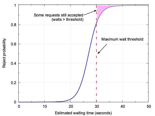
In the previous section, we saw a “hard cap” policy: if the expected wait exceeds a threshold, all new requests are immediately rejected. While this guarantees the queue never grows unbounded, it introduces an abrupt transition—one extra request can tip the system from accepting all to rejecting all, causing sudden drops in success rate (“cliff effect”) and making the user experience unpredictable around the threshold (see Figure 2).
For greater adaptivity and smoother user experience, we can make this process adaptive and robust to estimation error by applying a soft admission function—specifically, a sigmoid (also called logistic) curve. Here is how it works:
- The system still estimates the expected wait for a new request.
- Instead of
accept if wait < T, else reject, we compute a probability of acceptance that transitions smoothly from 1 to 0 as the predicted wait crosses the threshold. - Below threshold (say 20 seconds), most requests are accepted. Above threshold, requests are increasingly likely to be rejected.
- The transition region is tunable (by changing the sigmoid “slope” parameter), allowing for either sharper or softer cutoffs.
Figure 3 illustrates this behavior.
2.1. Why use a sigmoid for admission decisions?
At first glance, this might seem like a minor tweak, but employing a sigmoid function fundamentally enhances the system’s adaptivity and robustness:
- Graceful overload handling: Even when traffic exceeds capacity—whether just slightly or by multiples (e.g., 2× or 4× the nominal capacity)—a fraction of requests is still admitted. This mechanism not only absorbs minor bursts and compensates for estimation noise, but also helps mitigate larger surges and sustained overload conditions.
- Smooth user experience: Instead of a sudden rejection, the chance of being turned away increases gradually, making delays feel less abrupt and more understandable.
- Self-tuning: As traffic or system capacity shifts, the admission curve naturally adapts—allowing more users when conditions improve without needing manual adjustments.
- Resilient to estimation error: Rather than a strict yes/no decision, small errors in wait time predictions only affect the pace of admissions, not an all-or-nothing outcome.
- Backpressure, not blockage: Even when beyond the threshold, a random chance for entry is preserved, mitigating thundering herd effects and ensuring fairness.
📈 How queue size evolves under different loads
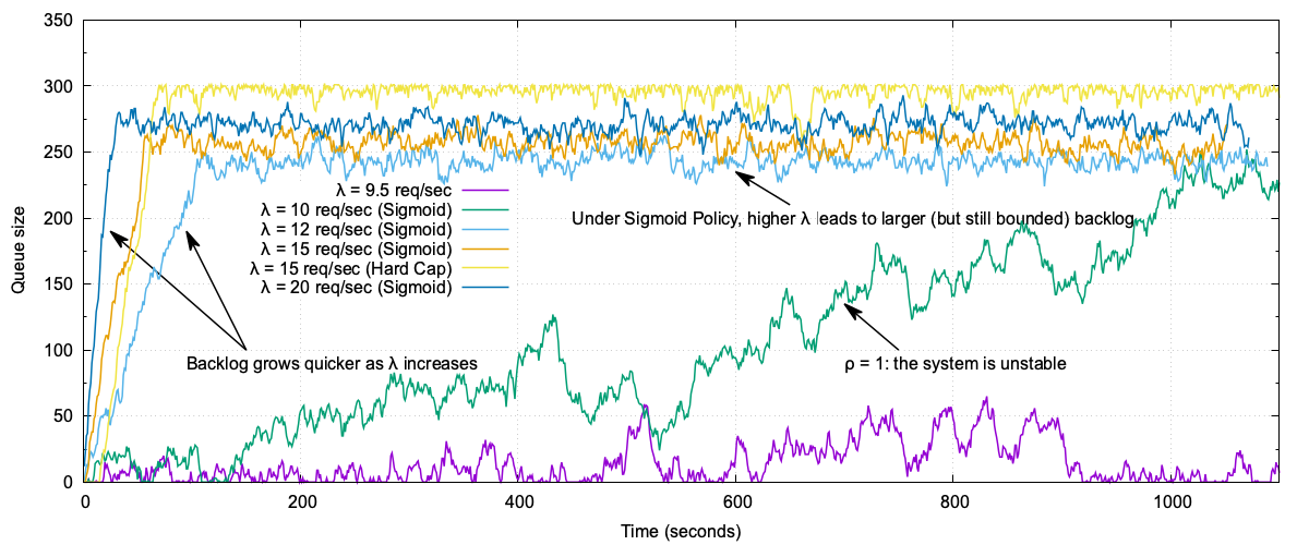
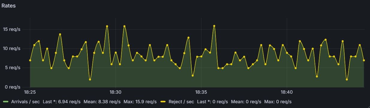
Our 20-minute test varied the arrival rate from 95% to 200% load (10 servers, mean service time = 1 s, Markovian traffic). Here is what we observed:
- At 95% load, the queue is manageable, with occasional backlogs (~50 jobs) that quickly drain.
- At 100% load, the system becomes unstable and the queue builds up gradually.
- At higher loads (120%–200%), backlog increases more rapidly as arrival rate rises.
Comparing admission policies at arrival rate = 15 (150% load, 30 s wait threshold):
- Hard cap: Queue quickly grows to ~300 jobs and remains fixed, with minor dips during brief load reductions.
- Sigmoid: Queue is bounded between ~230 and ~270 jobs, adapting more smoothly to traffic.
At arrival rate = 12, the queue is smaller than at 15. Notably, at arrival rate = 20 (sigmoid), the backlog is smaller than at 15 (hard cap) due to the sigmoid policy being more aggressive than the hard cap (it rejects some traffic also when the expected waiting time is smaller than T).
The chart below shows how queue size evolves for different overload levels. Under moderate overload, the system absorbs bursts with a “softer landing.” At extreme overload, almost everything is rejected, so the queue remains bounded. This adaptivity is more forgiving to spikes and robust against estimation error.
Implications
- Predictable but adaptive: The queue never grows fully unbound, but varies smoothly as overload increases.
- Tunable user experience: Adjusting the sigmoid’s steepness controls how sharply admission tightens under stress.
- Continuous feedback: Users see longer waits and a higher chance of rejection, but not a sudden all-or-nothing cutoff.
For the mathematically curious
As overload increases, the expected fraction of time a request is admitted depends on both the traffic rate and the exact sigmoid parameters. Unlike a hard cap (where max queue = constant), the sigmoid pre-filter regulates the queue at a level that depends on how far above capacity the demand gets—and how soft or sharp the probability function is. This means the queue size is not a fixed ceiling, but a dynamic, load-dependent value.
3. Should we add a hard cap?
The sigmoid admission control curve is highly effective for smoothing out sudden overloads and keeping queue size near a safe threshold. But in rare, extreme scenarios—massive surges or black swan events—even a small probability of admission can overwhelm backend resources.
A critical limitation of relying solely on the lobby service is that it must parse and process every incoming request, even when the system is clearly overloaded and most /join requests will be rejected. This can quickly lead to socket exhaustion, high CPU usage, and degraded stability—especially under heavy traffic or attack.
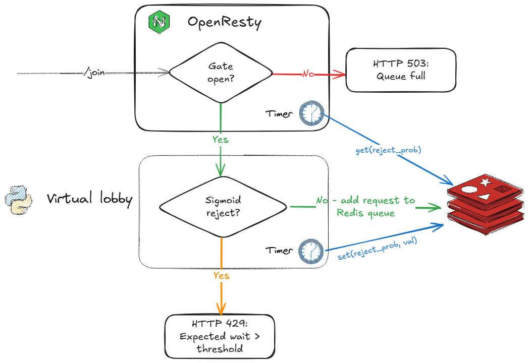
This is where our edge protection comes in, powered by OpenResty (think of it as Nginx “on steroids,” thanks to its LuaJIT engine for deep customization). Acting as a smart pre-filter, OpenResty intercepts traffic before it reaches the backend, reducing unnecessary load and protecting system resources. The mechanism works as follows:
- Our lobby service computes the current sigmoid reject probability once per second and stores it in a Redis key.
- OpenResty uses a timer to fetch this value from Redis every second, caching it locally.
This design choice is intentional: Redis acts as the single source of truth for admission control state, decoupling edge logic from backend implementation details. In our architecture, only the elected leader among lobby service processes updates the reject probability in Redis, ensuring consistency even when scaling horizontally. Admission decisions for/joinrequests are made atomically within Redis using Lua scripts, not in Python code—so it’s natural for OpenResty to fetch the latest value directly from Redis, guaranteeing that all components operate on the same, up-to-date state. - A custom Lua module applies hysteresis to avoid instability:
- If reject probability < 0.4: the gate is open—forward all traffic to the lobby service.
- If reject probability > 0.8: the gate is closed—return HTTP 503 to new requests.
- If reject probability is between 0.4 and 0.8: admit a fraction of traffic proportional to the reject probability, but always allow at least 10% through.
- The gate parameters (thresholds) can be changed at runtime via POST requests: our Nginx configuration exposes two custom endpoints,
/set_gate_thresholdsand/get_gate_thresholds, to update and retrieve the current values.
This dynamic, feedback-driven approach prevents overload, avoids abrupt cutoffs, and ensures the system remains resilient—even under extreme conditions. The OpenResty layer acts as a robust fallback and adaptive gatekeeper, keeping the backend healthy and responsive. When scaling horizontally (e.g., by running more gunicorn processes), this pattern continues to work seamlessly, as the edge logic and Redis state remain consistent across all backend instances.
In practice, OpenResty’s flexibility offers several additional benefits:
- Security: While this POC does not focus on security, Nginx/OpenResty can easily be configured to limit requests per IP address, block abusive clients, and mitigate DoS attacks at the edge.
- Observability: All gate metrics and thresholds are exposed via VictoriaMetrics and Grafana dashboards, making it easy to monitor, alert, and tune the system in real time.
- Extensibility: Lua’s power enables rapid customization. For example, we use a lightweight custom healthcheck module that returns HTTP 502 if the backend is unhealthy—much simpler than the standard
resty.upstream.healthcheckmodule. This approach allows for future enhancements, such as more granular traffic shaping or additional custom features as needed.
From a latency perspective, this edge logic adds negligible overhead: in our dockerized environment, the end-to-end latency measured by OpenResty—including the ASGI server and Redis—averages less than 2 ms, with 99th percentile latency in the 5-10 ms range. The system remains highly resilient without sacrificing responsiveness.
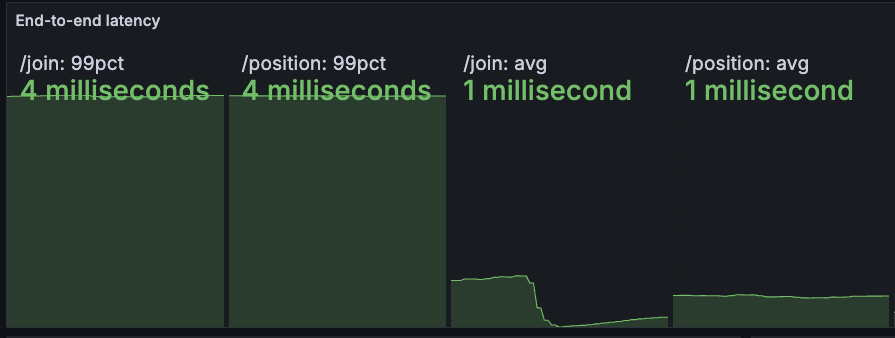
/join and /position endpoints, confirming sub-10 ms performance under load.💡 Optimized admission control pattern
4. Isolate failure domains
While edge protection and adaptive admission control guard against overload at the system boundary, it’s equally important to ensure internal reliability. To prevent surges in user traffic from impacting critical background operations, we isolate Redis clients by purpose:
r_user: user-facing connection poolr_internal: core system connection pool (internal components must never starve)r_pruner: small connection pool for background tasks (e.g., queue sampler, pruner)
The connection pools are configured to block rather than fail if no connection is available, and use exponential backoff for retries. This design prevents user bursts from starving workers and background tasks, ensuring robust operation even under stress.
from redis.asyncio import BlockingConnectionPool
from redis.backoff import ExponentialBackoff
from redis.retry import Retry

retry = Retry(ExponentialBackoff(cap=2, base=0.1), 3)
pool = BlockingConnectionPool.from_url(REDIS_URL, max_connections=5, timeout=1, decode_responses=True)
r = Redis(connection_pool=pruner_pool)
5. Reduce network activity
Minimizing network activity is a key tactic for robust overload protection. By reducing Redis commands and optimizing data access patterns, we keep the system responsive and scalable under stress. For a deeper dive into implementation details—such as atomic Lua scripts, local caching, and endpoint design—see our previous article: Implementing the Lobby Service with Redis.
This efficiency is especially important for the baseline validation that follows, ensuring that our measurements reflect true queueing behavior rather than network overhead.
Part F – Production readiness preview
This section presents a basic test, aimed at validating that our system performs as the math suggests. For this baseline, we bypassed OpenResty and disabled admission control—ensuring that every request is processed by the backend, without any filtering or gating. This allows us to directly compare observed queueing behavior against theoretical predictions (Erlang‑C).
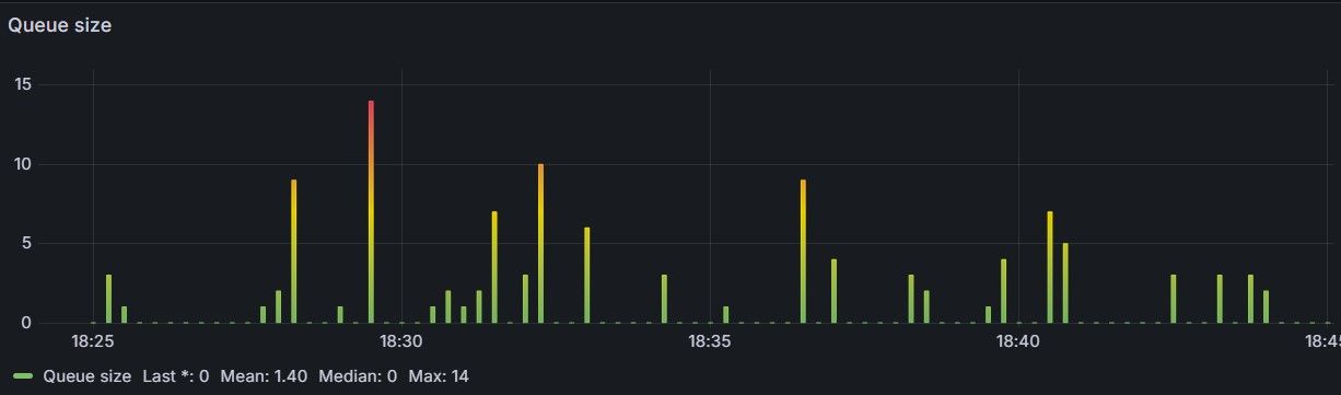
To calibrate the system, we used a ~100‑line Python asyncio script that fires λ = 8 requests per second on average (Figure 6), and ran it for 20 minutes. During that time, 9,574 requests went through the system. With 10 workers (μ = 1 req/sec), the Erlang‑C model predicts a mean wait of 0.191 seconds.
🛎️ For calibration, be sure your load generator is Poisson (use exponential inter‑arrival sleeps) so measured waits line up with Erlang‑C. Deterministic arrivals halve the variance and make the system look unrealistically good.
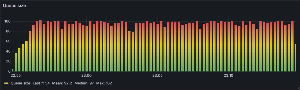
As can be seen in the table below, the observed waiting time is approximately 0.18 seconds, while the average queue size of the Redis queue stays around 1–2 (albeit with temporary spikes due to the random nature of the workload, see Figure 7), confirming the maths (results are inside sampling noise for ~10k requests and timer granularity).
| Metric (20 min run @ λ 8 req/sec) | Observed | Erlang‑C (c = 10, μ = 1, ρ = 0.8, cs²=1, ca²=1) |
|---|---|---|
| Mean service time | 0.998 s | 1.00 s (by design) |
| Mean queue wait | 0.179 s | 0.191 s (steady‑state) |
| p90 queue wait | 0.629 s | ≈ 0.67 s |
| p99 queue wait | 1.584 s | ≈ 1.82 s |
| Avg. queue length | 1.4 tokens | λ · E[w] ≈ 1.53 tokens |
Note: cs² and ca² are the squared coefficients of variation for service and arrival times, respectively. For Poisson arrivals and exponential service, both equal 1.
📌 As we mentioned in the first article, we enable uvloop when it’s available
try: import uvloop; asyncio.set_event_loop_policy(uvloop.EventLoopPolicy())
except ImportError: pass
On Windows (where uvloop doesn’t ship) the import fails and we try to use winloop — but the code runs with the standard asyncio loop too.
This baseline validation confirms that our queueing logic matches theoretical expectations under controlled conditions. In the next article, we will push the system further with stress tests and advanced performance evaluation.
6. Performance tuning: keep-alives and TIME_WAIT cleanup
Network-level details can have a surprising impact on queue performance and measurement accuracy. Even with a perfectly tuned backend, transport artifacts can distort results and degrade reliability.
When we switched our benchmarking client to close HTTP connections immediately after each /join (via Connection: close header), two side-effects emerged:
- Thundering
TIME_WAITsockets: eachConnection: closerequest forces the TCP stack to close the socket after response. That triggers a 4-way FIN handshake, after which the socket enters theTIME_WAITstate (typically 60 seconds on Linux). Over a long run at 50 joins/sec, our client and OS ran out of ephemeral ports, choking new requests. - Biased interarrival statistics: the OS-level TCP teardown latency crept into our interarrival timestamps, inflating the measured ca² well above 1—even though we were using a true Poisson process.
The fix
- Re-enable HTTP keep-alives on the client: with this setting enabled, each client opens a handful of persistent sockets instead of thousands of short-lived ones.
- Bump Uvicorn’s keep-alive timeout: the default Uvicorn
timeout_keep_aliveis 5 seconds. Increasing it to 60 seconds prevents Uvicorn from closing idle connections too quickly, avoiding premature TCP teardowns while the client is waiting in line.
uvicorn.run("lobby:app", host="0.0.0.0", port=8000, reload=False, timeout_keep_alive=60)These optimizations ensure that our queueing benchmarks reflect true system behavior, not artifacts of the underlying transport. With the right tuning, you can trust your measurements and keep your system robust under load.
Conclusion
In this article, we hardened our virtual queue for production by implementing adaptive admission control, edge protection, failure domain isolation, and network optimizations. These engineering choices ensure the virtual queue remains robust, responsive, and predictable—even under stress. We validated the system’s baseline performance against queueing theory, confirming that our implementation matches mathematical expectations under controlled conditions.
In the next and final installment, we will go beyond the baseline and subject our system to a series of stress tests under a variety of traffic patterns—including bursty loads, heavy tails, and sustained overloads. We will show how OpenResty and the sigmoid controller work together to keep the system stable, even when overloaded by more than 10× its nominal capacity. Detailed Grafana charts will illustrate how traffic is filtered and resilience is maintained under real-world pressure.
📬 Get weekly queue insights
Not ready to talk? Stay in the loop with our weekly newsletter — The Queue Report, covering intelligent queue management, digital flow, and operational optimization.