· Michele Mazzucco · 19 min read
Virtual queues from scratch, Part 3: ticket flow and liveness protocol
Part 3 of our hands-on series: learn to simulate realistic backend traffic patterns for robust testing, and implement a resilient liveness protocol to manage ticket lifecycles and automatically prune abandoned sessions in your virtual queue.

Missed Part 2? Catch up here.
In our “Virtual Queues from Scratch” series, we have steadily progressed from abstract concepts to a functional component. Part 1 laid down the architectural blueprint and core principles of virtual queues. Then, in Part 2, we brought the design to life by implementing our lean Python ASGI Lobby Service, leveraging Redis for robust state management. We now have a running service capable of receiving and holding users in a waiting room.
However, a virtual queue isn’t just about holding users; it’s about validating its behavior under realistic conditions and meticulously managing the state and validity of each user’s ticket within the system. This demands rigorous testing and a precise understanding of the ticket lifecycle.
In this third installment, we shift our focus to hardening our virtual queue for the real world through simulation and precise ticket management. We will first show you how to simulate backend services using Python coroutines, a powerful approach that allows us to thoroughly test our queue in isolation under a wide range of traffic conditions—from bursty peaks and heavy-tailed distributions to extreme overload scenarios.
More critically, this article dives deep into the core mechanics that ensure the queue’s reliable operation:
- The complete ticket lifecycle: Understanding a user’s journey from obtaining a token (a ticket) and entering the queue, through the process of remaining active, to either being successfully dispatched or having their ticket expire due to abandonment.
- The liveness protocol: Implementing the essential mechanisms for ticket lifetime renewal (via status updates) and the robust detection and pruning of expired/abandoned tickets, ensuring our queue remains accurate, efficient, and free of stale entries.
Note: In this series, we use the terms ticket and token interchangeably. Both refer to the unique identifier assigned to each user/session in the virtual queue. Whether we say “ticket” or “token,” we mean the same thing: the object that represents a user’s place and state in the queue.
Get ready to build a virtual queue that’s not just functional, but also intelligent, thoroughly tested, and optimized for managing every ticket with precision. In Part 4, we will then tackle crucial backend protection mechanisms, including dynamic admission control, to safeguard the system under the heaviest loads.
Table of contents
- Part C: Simulating backend services
- Part D: Advanced queue management
- Conclusion: a resilient queue takes shape
Part C: Simulating backend services
1. Why this approach is realistic and powerful
As promised at the end of our previous article, a crucial step in validating our virtual queue is to simulate the backend services it protects. This isn’t just a “toy” setup; it’s a powerful, battle-tested methodology used in various performance engineering and queuing theory studies. Hence, this straightforward Python coroutine approach offers high fidelity and realistic testing.
from typing import Protocol, Awaitable, Any

class WorkerRoutineFn(Protocol):
    def __call__(self, ctx: AppContext, *args: Any, **kwargs: Any) -> Awaitable[float]:
        ...

async def sleep_routine(ctx: AppContext, *args: Any, **kwargs: Any) -> Awaitable[float]:
    # Create random service time according to a distribution of choice
    svc_time = ctx.service_times_prng.generate_deviate()
    await asyncio.sleep(svc_time)
    return svc_time

async def worker(idx: int, ctx: AppContext, routine: WorkerRoutineFn = sleep_routine):
  redis: Redis = ctx.get_redis_internal()
  while True:
      task = await redis.blpop("lobby:queue", 0) # Block if the queue is empty
      # Update statistics, perform validation, ...
      svc_time: float = await routine(ctx) # Execute task
      # Update statistics ...
This deceptively simple code forms the backbone of our backend simulation. Each Python coroutine acts as an independent worker, mimicking a real backend service. It patiently waits for a user request (a “task”) from the Redis queue using BLPOP (a blocking operation that perfectly reflects a worker waiting for work). Once a task is received, it simulates processing that task by “sleeping” for a configurable amount of time.
This is realistic and an effective strategy to test how our virtual queue behaves:
- Mimicking real-world latency and throughput: Real backend services aren’t instantaneous. They process requests over time. By introducing a sleep based on a random distribution, we accurately model the latency a real request would experience and, consequently, the throughput of our simulated backend. This is fundamental to understanding queue behavior.
- Emulating diverse workload patterns: The power lies in
ctx.service_times_prng.generate_deviate(). This isn’t a fixed sleep time; it’s a random number generator configured to follow specific statistical distributions. This allows us to realistically simulate:- Constant workload: If
svc_timeis fixed. - Variable workload: Using uniform or normal distributions.
- Realistic backend processing: Using more complex distributions like exponential, Pareto (heavy-tailed), or log-normal distributions. While our experiments in this series will focus on Markovian traffic and heavy-tailed traffic modeled with log-normal distributions (exploring different squared coefficients of variation), nothing prevents readers from experimenting with other traffic patterns like fixed, normally distributed, or Pareto.
- Transient conditions: By dynamically adjusting the distribution parameters, we can simulate changes in backend performance, such as slowdowns or temporary bottlenecks.
- Constant workload: If
- Resource contention (implicit): While these workers aren’t consuming CPU cycles on actual database queries, their rate of consumption from the queue effectively models the backend’s capacity. If workers are slow (high
svc_time), the queue grows; if they are fast, it drains. This indirectly simulates resource contention within the backend. - Isolation for focused testing: By controlling the backend’s behavior precisely, we can isolate the queue’s performance from external factors. This allows us to focus purely on how our virtual queue handles different load profiles and validate its internal logic, liveness detection, and admission control mechanisms without interference from complex, unpredictable downstream systems.
- Scalability testing: We can easily spin up many of these coroutines to simulate a large backend farm, pushing our virtual queue to its limits in a controlled environment.
This simulation strategy is a cornerstone in fields like queuing theory, operations research, and performance testing. Many professional load generators and simulation frameworks, while offering more sophisticated features, fundamentally rely on this same principle of simulating service times or suspend execution to model downstream system behavior accurately. It provides a robust and repeatable way to validate our queue’s resilience long before it faces real-world traffic.
🛎 How about executing a real task?
Deep dive: modeling traffic variability for realistic simulation
Understanding how to accurately model incoming traffic and service times is paramount for truly effective queue testing. Real-world systems rarely experience perfectly uniform loads; instead, they contend with bursts, unpredictable spikes, and heavy-tailed service distributions that can disproportionately impact performance. Below, we will delve into the nuances of simulating this variability, including common pitfalls and key rules of thumb to ensure your tests reflect actual operational challenges. We will explore concepts like:
- Mean vs. median,
- Distribution shape (CDF and PDF), and
- The critical role of outliers in system behavior.
📊 Click to expand: The art and science of traffic modeling
📈 Real-world traffic variability: what it really looks like
Real world traffic doesn’t follow text-book models. Hence, we need a clear metric for variability. The most practical one is the squared coefficient of variation (SCV, or cv2), which is defined as the variance divided by the squared mean:
Why use SCV?
- It is normalized by the mean: you can compare distributions with wildly different scales.
- It is easy to compute in real time: just track sum, count, and sum of squares—perfect for efficient storage in Redis.
🎯 Interarrival time SCV (traffic burstiness)
In the real world, arrivals are rarely Poisson. Traffic is bursty, spiky, and comes in waves or batches. Here are some common scenarios and SCV estimates:
| Scenario | SCV estimate | Notes |
|---|---|---|
| Call centers (steady hours) | ~1.0–2.0 | Some overdispersion, mild bursts |
| Retail/online flash sales | 5.0–20.0+ | User rush causes spikes |
| Government service sites (opening hour) | 4.0–10.0 | Morning spikes or deadline surges |
| Concert ticket launches | 10.0–50.0+ | Users flood in at exact release time |
| Social media-driven traffic | 20.0+ | Influencer links, viral posts |
📌 Rule of thumb:
Anything with coordinated user behavior (time-based triggers, social media, deadlines, etc.) will show high SCV (≫ 1) in interarrival times.
🎯 Service time SCV (how variable is each request)
The service time (how long each request actually takes) depends on what the system is doing and who is involved:
| Scenario | SCV Estimate | Notes |
|---|---|---|
| Simple transactions (API ping, login) | ~0.5–1.0 | Mostly consistent |
| Form submissions with validation | 1.0–2.0 | Some users take longer, retries |
| Complex tasks (payment, ID checks) | 2.0–5.0 | Varies by input, edge cases |
| Call center conversation lengths | 2.0–10.0 | Long-tail talk durations |
| Virtual waiting room (CAPTCHA, retries) | 2.0–8.0 | Depends on user/device/browser variance |
📌 Rule of thumb:
If user interaction or external dependencies are involved, SCV of 2–5 is realistic—but can be much higher in special situations.
🔎 What does this mean in practice?
To examine real-world burstiness, we will look at two models beyond “textbook exponential”: the lognormal (continuous, multiplicative randomness—think file sizes, latency tails) and the hyperexponential (the classic Markov “two classes of jobs” scenario). Both can have identical average and SCV, but their tail behavior—and impact on your system—is radically different.
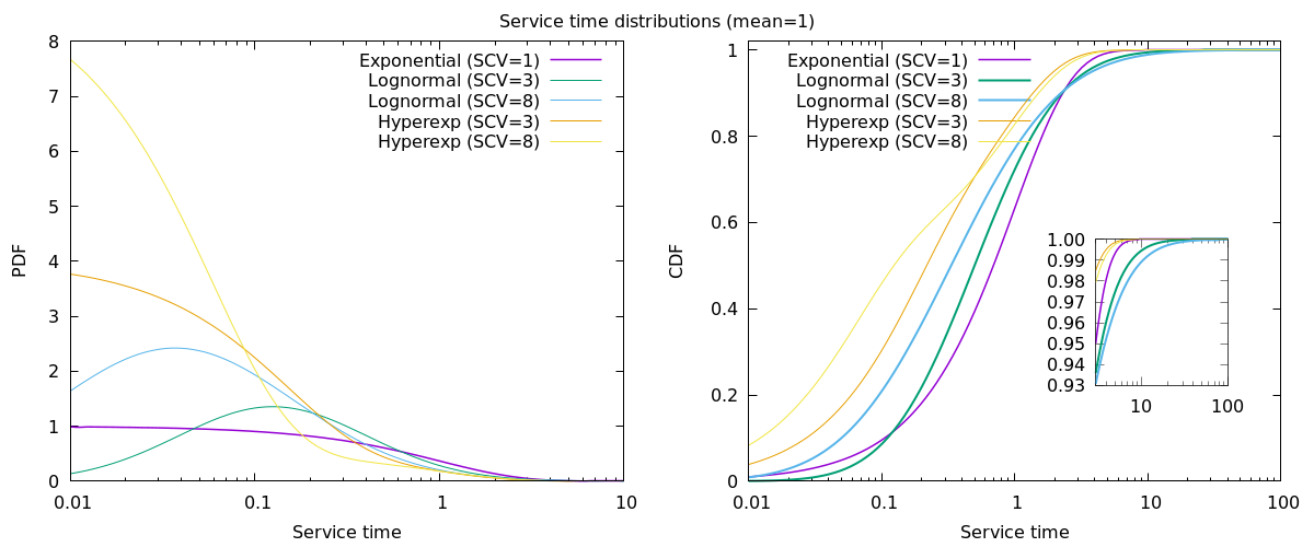
Distribution Shapes: PDF and CDF
Below, we plot the probability density (PDF, left) and cumulative distribution (CDF, right) for each distribution, with different SCV values:
- Exponential (SCV=1): Textbook, memoryless, “boring” traffic
- Lognormal (SCV=3, 8): Typical for real-world heavy-tailed workloads
- 2-phase hyperexponential (SCV=3, 8): “Bursty,” with a mix of many small and rare big values
All have mean = 1 for easy comparison.
Notice how the fraction and scale of big outliers changes, even when the mean and SCV are the same.
🔎 Why does hyperexponential shift to the left?
How bad are the outliers?
When you sample from heavy-tailed distributions, you will get some surprisingly large values—even if the mean is equal to 1.
But not all outliers are created equal:
- Hyperexponential bursts are “rare but respectable”—big, but with a natural cap.
- Lognormal outliers are “rare and wild”—the biggest one could be shockingly, even catastrophically larger than all the rest.
Here is what you can expect for a batch of 10,000 requests:
| Distribution | SCV | Typical maximum (outlier) |
|---|---|---|
| Exponential | 1 | ln(n) ~10 |
| Lognormal | 3 | 60–150 |
| Lognormal | 8 | 400–2,000 |
| Hyperexponential | 3 | 30–60 |
| Hyperexponential | 8 | 120–200 |
Why does this happen? Even when two distributions have the same SCV (burstiness), how they “package” their tail risk is very different:
- Lognormal: Spreads out that tail chance over an incredibly wide range of values. Most requests are modest, but a few might be 10, 100, or even 10,000× the mean.
- Hyperexponential: Packs all tail risk into a rare “slow” phase. These jobs are still far bigger than the mean, but the chance of going much beyond that is close to zero.
TL;DR:
The outlier probability is similar, but the worst-case size is radically different. Lognormal can produce black swan requests that dwarf anything you will see from a hyperexponential with the same SCV.
Simulating realistic variability: pitfalls and proper truncation
Heavy-tailed distributions (like lognormal with high SCV) converge very slowly:
- Even with a million samples, your observed SCV can fluctuate by ±20% or more.
- For 10,000-100,000 samples (a realistic demo workload), outliers can dominate the SCV—and every batch will look a little different.
- If you get (or don’t get) even one of those rare huge samples in your batch, it drastically affects the sample variance.
⚠️ Shortcuts and pitfalls: capping, resampling, and the right way to simulate outliers
When simulating highly variable workloads (like ticket lobbies), two common shortcuts are:
- Resampling: If a randomly drawn service time exceeds your cap, simply redraw until it doesn’t.
Pitfall: This “trims” outliers, but almost always replaces rare big values with frequent small ones, lowering the average and variability below your targets. - Hard capping: If a value is above the cap, set it exactly to the cap (e.g.,
service_time = min(lognormal(), cap)).
Pitfall: This prevents runaway outliers, but creates an unnatural spike (“bump”) at the cap. The resulting distribution is no longer lognormal or even smooth.
Both tricks break the link between your chosen parameters and the actual (mean, SCV) of your simulated workload.
The sample variability and average will no longer match what you intended—making system tests less meaningful.
The correct approach relies in mathematically calibrate the truncated distribution:
- Pick the cap you want (e.g., 30 seconds).
- Solve for parameters so the mean and SCV of the capped distribution hit your targets (e.g., by tuning σ using a bisection method).
- Draw values, capping and resampling only as needed.
With this, the test workload is both realistic and controllable: you get high variability, but avoid “unlucky” outliers that would swamp the queue.
Key takeaways:
- Real traffic is far more variable—and risky—than the classic textbook models suggest.
- Always model, measure, and expect variability, not just averages.
Part D: Advanced queue management
In this section, we will discuss the handling of abandoned tickets (i.e., users leaving the system).
2. The Liveness system: status updates and abandonment detection
A key challenge in any lobby service is managing the constant stream of requests from clients wanting to know their status (“What’s my position in line?”). This polling mechanism, while essential for user experience, serves two critical and simultaneous functions:
- Status updates: It provides real-time feedback to the user.
- Liveness signal: It acts as an implicit “proof of life” or heartbeat, allowing the system to detect users who have abandoned the queue.
This duality presents two distinct engineering challenges: one of performance at scale, and one of accuracy in abandonment detection. This section explores both challenges and details the unified solution our POC implements to solve them.
2.1. The Performance challenge: managing polling at scale
Even if the primary /join endpoint is throttled, the status polling endpoint (e.g., /position/{token}) can easily become a new performance hotspot. The load on the system is a function of the queue size and polling frequency. As the queue grows, the problem compounds:
- Longer queues mean more users are waiting.
- Longer waiting times mean each user will make more polling requests during their session.
- Each poll triggers backend operations, such as Redis calls, consuming connections from a limited pool.
For a small queue of a few hundred concurrent visitors, polling every second is perfectly safe. However, the load does not scale linearly.
| Lobby size | Poll 1 sec. | Poll 2 sec. | Why you’d change |
|---|---|---|---|
| ≤ 1k waiting | 1k rps, ~1k sockets | 500 rps | Trivial load, often < 1% CPU |
| ≈ 10k waiting | 10k rps, 10k sockets | 5k rps | Risks hitting default file-descriptor limits on the server. (1024 / 4096) |
| > 50k waiting | 50k rps, 50k sockets | 25k rps | Can consume a full vCPU core just handling poll requests |
Clearly, a naive, fixed-rate polling strategy creates a significant scaling problem.
2.2. The Liveness challenge: pruning abandoned sessions
While managing performance is critical, the liveness signal provided by polling is equally important. For a busy lobby service, failing to efficiently handle user abandonment leads to:
- Wasted processing resources when users are eventually served.
- Skewed queue-time statistics and inaccurate estimates.
- A degraded experience for active users forced to wait behind “ghost” sessions.
The system needs a reliable way to identify and remove users who are no longer waiting.
In high-demand scenarios (e.g., trying to buy a ticket for the UEFA Champions League final), the time a user spends waiting in the queue can be orders of magnitude longer than the time spent in active processing. Therefore, accurately managing abandonment from the queue is the most critical aspect for ensuring system stability and fairness.
For the scope of this POC, we focus exclusively on this challenge. We assume that users only abandon the system while waiting in the queue. This simplifying assumption allows us to rigorously test the core lobby service mechanics, and the results remain highly valuable. The more complex scenario of in-flight abandonment is discussed in Section 5.2 as a key consideration for a fully productionized system.
2.3. The unified solution: dynamic grace periods and adaptive polling
We solve both the performance and liveness challenges with a single, elegant mechanism: a dynamic grace period for polling.
Instead of allowing clients to poll at a fixed interval, the system instructs the client on how long to wait before its next poll. This duration is unique to each session and depends on its real-time position in the queue as well as on how fast the queue moves.
The logic is simple yet powerful:
- Users at the back of the queue receive a long grace period. A user who has a long wait ahead does not need to prove their presence as frequently. This dramatically reduces the total number of heartbeat requests handled by the system.
- Users nearing the front of the queue receive a much shorter grace period. As a user’s turn approaches, the system requires a higher-confidence signal that they are still present. This minimizes the probability of a backend worker pulling a request for a user who has just abandoned their session.
An example of how to compute the polling interval based on our algorithm is given by the code snipped below.
from random import uniform

def compute_poll_interval(w: float, std_wait: Optional[float] = None, *,
        min_poll: float, max_poll: float, k_far: float, k_near: float, threshold: float) -> float:
    """
    Compute the recommended polling interval.
    Use more aggressive polling as jobs near the front, more lazy when far.
    """
    if std_wait is None:
        std_wait = 0.0

    poll = (w + std_wait) / (k_near if w < threshold else k_far)
    poll = max(min_poll, min(poll, max_poll))
    # Add a small jitter to avoid sync
    poll *= uniform(0.9, 1.1)
    return poll
This self-throttling approach elegantly resolves both challenges:
- It solves the performance problem by dramatically reducing the overall number of poll requests from users deep in the queue, keeping server load flat and manageable.
- It solves the liveness problem by ensuring the highest-fidelity signal is received from users who are about to consume backend resources, minimizing waste.
The server communicates the next polling interval to the client via a simple HTTP header in the status response (e.g., x-poll-after-seconds: 60), which the client can use to adjust the polling frequency:
$ curl -i http://localhost:8000/position/bdea74e6-5c19-40c0-9fc3-fef8cc0a7485
HTTP/1.1 200 OK
x-poll-after-seconds: 14.33
...

{"position":318,"wait":28.82,"variance":4.45}
As the user moves towards the front of the queue, the estimated waiting time decreases, as does the value stored in the x-poll-after-seconds header, reflecting the need for more frequent liveness checks:
$ curl -i http://localhost:8000/position/bdea74e6-5c19-40c0-9fc3-fef8cc0a7485
HTTP/1.1 200 OK
x-poll-after-seconds: 2.19
...

{"position":62,"wait":5.33,"variance":1.96}
📌 In production we would either
- a) open more Uvicorn workers
- b) push readiness via WebSocket/SSE, or
- c) throttle polling to once every few seconds, either using
CL.THROTTLE(if using Dragonfly) or a Lua script.
2.4. Queue-pruning details
To act on this liveness data, the system must efficiently remove expired sessions. Our implementation achieves this without scanning the entire queue by using two Redis Sorted Sets (ZSETs):
lobby:pending: Stores user IDs, scored by their entry timestamp (for FIFO order).lobby:expiry: Stores the same user IDs, scored by last-seen time (updated on each successful poll).
A small, periodic Lua script runs on the Redis server to efficiently prune expired tokens from the queue. It begins by performing a ZRANGEBYSCORE on the expiry sorted set, retrieving all tokens whose last_seen_timestamp is older than their dynamic grace period. These expired tokens are then removed in batches from the relevant ZSETs using ZREM.
This entire pruning operation is extremely fast, with total time complexity O(M × log N), where N is the size of the ZSET and M is the number of expired (stale) entries processed in this run. Because the script runs frequently and typically only a small number of tokens expire per interval, both M and the resulting prune time are usually very low—ensuring that queue maintenance is highly efficient even as the workload grows.
Expired tickets are removed from the lobby:queue list by the workers once they reach the front of the queue, in O(1) time — this is not a problem, since we do not use this data structure for statistic purposes.
3. Handling in-flight abandonment
While the POC focuses on queue abandonment, a full production system must also consider users who leave while their request is actively being processed.
This scenario is typically solved with a Cancellation Token pattern, where a backend worker can be proactively notified that its current job should be terminated. The implementation depends on the nature of the job (e.g., graceful termination for read-only requests, a database ROLLBACK for transactional requests, or a Saga for long-running transactions).
Comparing liveness signaling patterns
The effectiveness of any abandonment model depends on the speed and reliability of the liveness signal. Here are three common patterns.
| Pattern | Description | Latency | Reliability | Complexity |
|---|---|---|---|---|
| Liveness polling (Heartbeats) | The client periodically sends an HTTP request. This can be a fixed-interval poll or a more sophisticated implementation like the Dynamic Grace Period model detailed in Section 4.3. | High | High | Low |
| Proactive signal (sendBeacon) | The browser sends a final message upon closing. This provides an early, proactive cancellation signal. The heartbeat remains as a fallback. | Low | Medium | Medium |
| Persistent connection (WebSockets) | The client holds a WebSocket connection open. A disconnect is an immediate, positive server-side event. This pattern is the highest performing but also the most complex. | Very Low | High | High |
A robust WebSocket implementation must handle temporary network glitches by using a reconnection grace period, which gives clients a short window to reconnect before their session is declared abandoned.
Real time communication solutions such as Pushpin, Nchan or Mercure, or message bus brokers like NATS can help here - however bear in mind that their deployment and configuration may be complex, depending on your setup.
Conclusion: a resilient queue takes shape
We have covered significant ground in this third part of our “Virtual Queues from Scratch” series. We began by establishing a powerful and realistic testing environment, leveraging Python coroutines to simulate backend services. This approach, backed by queuing theory principles, allows us to rigorously test our queue under diverse and challenging traffic patterns, including bursty and heavy-tailed distributions. We explored the nuances of modeling traffic variability, including concepts like the Squared Coefficient of Variation (SCV), probability distributions (PDF/CDF), and the critical impact of outliers and “black swans” on system behavior. We also discussed common pitfalls like improper truncation and the correct approach to ensure test workloads are both realistic and controllable.
With our robust simulation framework in place, we then delved into advanced queue management mechanisms vital for a production-grade virtual waiting room.
We meticulously defined the complete ticket lifecycle, illustrating a user’s journey from entry to dispatch or abandonment. Central to this was the liveness system, which tackles both the performance challenge of managing polling at scale and the accuracy challenge of detecting abandoned sessions. Our dynamic grace period solution elegantly solves these challenges by adaptively adjusting client polling frequency based on queue position. Furthermore, we detailed how efficient queue pruning is achieved using two Redis Sorted Sets and optimized Lua scripts, guaranteeing an accurate and performant queue at any scale.
Finally, we explored the critical consideration of handling in-flight abandonment for a fully productionized system, discussing patterns like cancellation tokens, sendBeacon, and WebSockets as superior alternatives to simple polling for liveness signaling.
We now have a virtual queue that is not only functional and well-tested but also equipped with intelligent mechanisms to manage user flow and maintain its integrity under demanding conditions. Stay tuned for Part 4, where we will build upon this foundation to implement crucial backend protection features, including dynamic admission control, to safeguard our system under the heaviest loads.
📬 Get weekly queue insights
Not ready to talk? Stay in the loop with our weekly newsletter — The Queue Report, covering intelligent queue management, digital flow, and operational optimization.