Santa's sleigh and the science of logistics: an optimization story

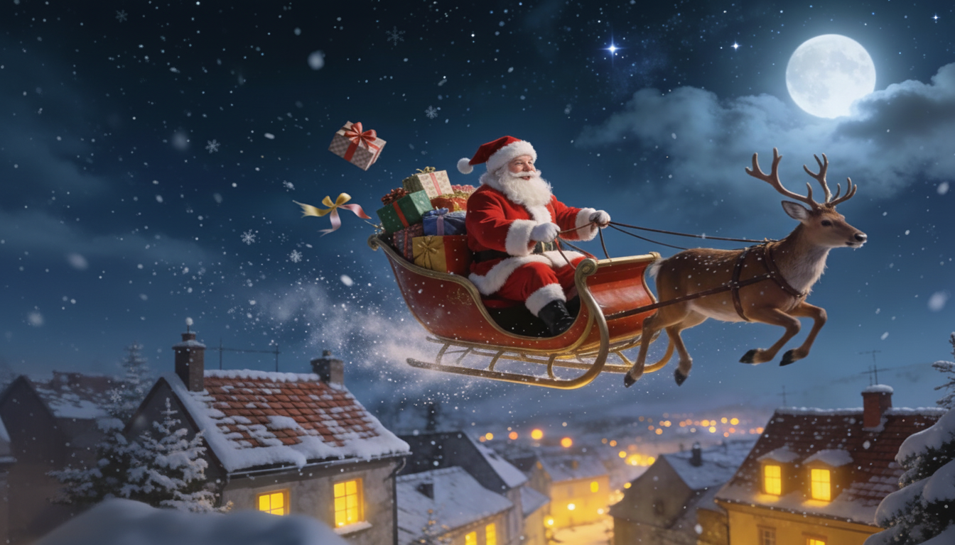
As we approach Christmas, it’s easy to get lost in the magic of the season. But at QueueworX, we look at the North Pole and see something else: the most sophisticated logistics operation in history.

We often talk about queueing theory, Little’s Law, and the psychology of waiting. But this week, I want to pivot to a vertical that keeps the world moving: Logistics Optimization. And who better to study than the ultimate fleet manager, Santa Claus?

While Santa has magic, he also has constraints. To deliver gifts to roughly 2 billion children in a single night, he faces a classic optimization challenge known as the Vehicle Routing Problem (VRP).

Table of contents

• The problem: A traveling salesperson on a deadline
• The math: Linear Programming the North Pole
  • The objective function
  • The constraints
• A tiny 5-kid example
• Heuristics in action
• Why it matters for real logistics
• Conclusion

The problem: A traveling salesperson on a deadline

If Santa had infinite time, this would be a standard Traveling Salesperson Problem (TSP): finding the shortest path to visit a set of cities (or chimneys) and return to the start.

But Santa operates under strict constraints:

• Time windows: He has about 31 hours (thanks to time zones and the rotation of the earth) to complete his rounds.
• Capacity: Even with a magical sack, there are limits to volume and weight (requiring potential “refills” at depots).
• Topology: He must visit every unique location exactly once.

The math: Linear Programming the North Pole

To solve this, we can’t just guess. We need Linear Programming (LP)—specifically, Integer Linear Programming (ILP). This is the same math used by FedEx, UPS, and DoorDash to optimize delivery routes.

Let’s define our variables. We create a binary variable $x_{i,j}$ where:

• $x_{i,j}=1$ if Santa travels directly from house $i$ to house $j$, and
• $x_{i,j}=0$ otherwise.

The objective function

Santa’s goal is to minimize total travel time (or distance). In optimization terms, we write this as:

$\text{Minimize Z} = \sum_{i} \sum_{j} c_{i,j} x_{i,j}$

where $c_{i,j}$ is the “cost” (time/distance) to travel between house $i$ and $j$.

The constraints

The “magic” (or the headache) is in the constraints. We must tell our model what is allowed:

1. Flow conservation (visit every house once): Santa must arrive at house $j$ from exactly one other location, and leave house $j$ to go to exactly one other location:

$\sum_{i} x_{i,j}=1$ for every $j$, and $\sum_{j} x_{i,j}=1$ for every $i$.

2. Subtour elimination: We must ensure Santa doesn’t get stuck in a loop visiting just three houses in Chicago while ignoring the rest of the world; the route must be one continuous tour connected to the North Pole. To enforce this in the math, we use subtour elimination constraints, such as the classic Miller–Tucker–Zemlin (MTZ) formulation, which assigns an order number to each stop and forbids disconnected mini-tours that violate this global ordering.

3. Time windows: Santa can only visit house $i$ during night hours. If $t_{i}$ is the arrival time at house $i$:

$Sunset_{i} \leq t_{i} \leq Sunrise_{i}$

A tiny 5-kid example

To see why Santa needs optimization at all, imagine a toy version with just 5 kids: Anna, Ben, Carla, Diego, and Emma, all living in different parts of the same town.

• Santa starts at the North Pole (a depot) and needs to visit each child exactly once, then return.
• Suppose driving between any two homes takes between 1 and 20 minutes, depending on distance.

Even with only 5 stops, the number of possible visiting orders is already $5! = 120$ different routes (fixing the North Pole as start/end). That’s small enough to check by hand or with a laptop.

Now scale this up:

• 10 kids: $10! = 3,628,800$ possible routes.
• 20 kids: $20! \approx 2.43 \times 10^{18}$ routes.

At Santa’s real scale—millions of stops—the brute-force approach is hopeless. Optimization models (like the integer programming model above) and smart heuristics become the only way to get a near‑optimal route in reasonable time.

Heuristics in action

To see a heuristic at work, let’s apply the nearest neighbor algorithm to our 5-kid example. The algorithm follows one simple rule:

• From your current location, always go to the closest unvisited stop next.

Starting at the North Pole (depot), the closest kid is Anna (say, 4 minutes away). From Anna, the closest unvisited is Ben (2 minutes). From Ben, Carla (2 minutes). From Carla, Diego (3 minutes). From Diego, Emma (4 minutes). Then back to the depot (5 minutes).

In summary:

• Total route: Depot → Anna → Ben → Carla → Diego → Emma → Depot.
• Cost: 4 + 2 + 2 + 3 + 4 + 5 = 20 minutes.

Is this optimal? Probably not (an optimal route might be closer to 18 minutes). But it’s fast to compute and gives a solid baseline. Is it useful? Absolutely—especially as a starting point you can improve with better heuristics.

Real logistics teams use this and many other heuristics to trade perfection for speed—getting high-quality routes quickly instead of waiting for exact solutions.

Why it matters for real logistics

Why do we care about Santa’s math? Because this is an NP-Hard problem. As the number of houses grows, the number of possible routes grows factorially. A computer trying to calculate every single option for 2 billion stops wouldn’t finish before the heat death of the universe.

But there is a more human reason this matters. In logistics, customers rarely experience “distance” or “constraints” directly — they experience uncertainty: When will it arrive? Am I forgotten? Why did someone else get served first? A better routing plan doesn’t just reduce miles; it improves predictability, which increases perceived control and fairness.

That is the queue-management connection: whether people are waiting in a line or waiting for a delivery, transparency and reliable time windows often matter as much as raw speed.

In the real world, logistics companies—and QueueworX clients—use “Heuristics” or “Meta-heuristics” (like Genetic Algorithms or Simulated Annealing) to find a good enough solution quickly. They trade perfection for speed, just like Santa might skip a second cookie to make up time.

Conclusion

Whether you are managing a global fleet or just a queue of customers at a coffee shop, the principles remain the same: minimize friction, respect constraints, and optimize the flow.

And when your goal is customer trust, remember: optimizing for predictability often beats optimizing for raw speed.

At QueueworX, we might not have reindeer, but we love tackling the math that makes operations fly.

Merry Christmas and happy optimizing

📬 Get weekly queue insights

Not ready to talk? Stay in the loop with our weekly newsletter — The Queue Report, covering intelligent queue management, digital flow, and operational optimization.