The hidden cost of variability: why reducing variance often beats reducing the mean

Photo by StockCake

If you run a contact center—whether a call center, a retail checkout, or a digital waiting room—you likely have a dashboard showing Average Service Time (often called AHT in most WFM/ACD tools, and written as $E[S]$ in queueing theory). And if you are like most leaders, you probably push your team to lower that number.

It seems intuitive: if each transaction takes less time on average, the line moves faster, right?

Wrong. In queuing systems, the average speed matters far less than the consistency of speed.

A system where every customer takes exactly 60 seconds will flow smoothly at 95% capacity. A system where customers average 60 seconds—but some take 10 seconds and others take 5 minutes—will collapse into gridlock at the same capacity.

This is the hidden cost of variability. It is the reason why adding staff often fails to fix wait times, and why “fast” teams can still have angry customers. In this article, we’ll look at the math that explains why variance is the enemy of flow, and why savvy operators focus on standard deviation before they focus on means.

Table of contents

• 1. The trap of averages
• 2. The physics of waiting (why 1+1 does not equal 2)
• 3. Evidence from the lab: The consumer of capacity vs The disruptor of flow
• 4. A practical example: the “heavy tail” in action
• 5. The strategic fix: reducing variance beats reducing mean
  • 5.1. Segmentation (the “express lane” is math, not just courtesy)
  • 5.2. Triage and “Shortest Job First”
  • 5.3. Hard caps (truncating the tail)
• 6. The ROI of stability
• Conclusion

1. The trap of averages

Imagine two coffee shops, both with a single barista. A contact center is the same system: each interaction “occupies” an agent for a service time, and new contacts arrive whenever customers decide to reach out.

• Shop A (the steady shop): Every customer takes exactly 2 minutes to serve.
• Shop B (the variable shop): Half the customers take 1 minute (drip coffee), and half take 3 minutes (complex lattes).

The average service time for both shops is identical: 2 minutes. If you look at a monthly report, both shops look equally efficient.

But physically, they behave completely differently. In Shop A, if a customer arrives every 2.1 minutes, the line never grows. The barista finishes one operational cycle just before the next customer arrives. Flow is perfect.

In Shop B, randomness destroys the flow. If three “latte” customers arrive in a row (taking 9 minutes total), but only 6 minutes of “arrival time” passes, a queue forms. The next “drip” customer—who should only take 1 minute—is stuck waiting behind the logjam.

This is the core insight of queuing theory: Queue size is not just a function of traffic volume; it is a function of variability.

2. The physics of waiting (why 1+1 does not equal 2)

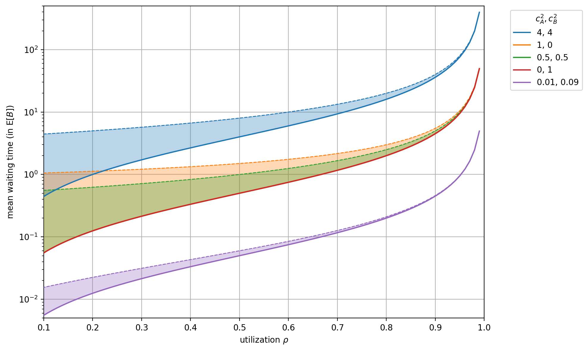
There is a formula for this, known as Kingman’s equation, developed in 1961: it gives us an approximation of the waiting time for G/G/1 queues (general arrival/service distributions, single server). While there is no need for you to memorize the equation, you should definitely memorize its implications. Roughly speaking, the expected average waiting time in a queue is determined by three factors:

$E[w] \approx \left(\frac{c_A^2 + c_S^2}{2} \right) \times \left( \frac{\rho}{1 - \rho} \right) \times E[S]$

where $c_A^2$ and $c_S^2$ are the squared coefficient of variation of interarrival intervals and service times, respectively (i.e., the variance divided by the squared mean), while $\rho$ is the system utilization (in contact-center language: agent occupancy). If $\rho >= 1$ the system is overloaded and both the queue and waiting times will grow unbounded. Hence, we require $\rho < 1$.

Note that $E[w]$ is the average time spent waiting before service starts, and not the total time the job spent in the system (which is the sum of waiting and service time).

The above formula is the product of three intuitive “multipliers”:

1. The variability multiplier captures how irregular your arrivals are ($c_A^2$) and how inconsistent your service times are ($c_S^2$). If your service process becomes twice as variable, waiting time roughly doubles—even if the average speed stays the same.

2. The utilization multiplier is the “running hot” penalty. As utilization approaches 1, the denominator $(1-\rho)$ shrinks and waiting time blows up. The same amount of variability that’s tolerable at 80% utilization can become catastrophic at 95%.

3. The scale multiplier is the baseline unit of work. All else equal, if every job takes 10% longer on average, the queue’s waiting time scales up with it.

The key operational takeaway is that you can attack wait times through three levers—stability, slack, and speed—but the “variance tax” is often the most underestimated. And because the utilization term is non-linear, variance hurts you most precisely when you are busiest—see Figure 1 below.

This explains a common operational mystery: “Why did our wait times spike today? We had the same number of customers as yesterday.” The answer is usually variability. A few “heavy” transactions clumped together, or a few staff members had inconsistent pacing. The average volume was fine, but the variance killed the flow.

This is why service levels can miss on “normal volume” days: a handful of unusually long contacts can absorb enough agent minutes to push everyone else into queue.

3. Evidence from the lab: The consumer of capacity vs The disruptor of flow

In our recent study on virtual queue performance, we didn’t just model this—we proved it in a controlled environment. We compared two systems pushing distinct traffic patterns through the same capacity:

1. Bursty arrivals: Traffic comes in waves (spikes), but service times are consistent (low variance).
2. Variable service: Traffic is steady, but service times vary wildly (high variance/heavy tails).

The result: System #2 (variable service) performed dramatically worse. Specifically, heavy-tailed service times caused median wait times to increase by nearly 10x compared to the baseline, and extreme “tail waits” (the 99th percentile) exploded.

One may wonder why the impact is so different.

• A burst of arrivals eventually clears as the team works through the pile, and because the work itself is consistent, they catch up.
• A slow service transaction effectively “breaks” the server. If one customer takes 10 minutes in a 1-minute line, that server is effectively offline for 9 minutes of excess time. Everyone behind them stops moving. This is known as head-of-line blocking.

Importantly, that experiment used a multi‑server system, not just a lone worker. We had multiple “agents” working in parallel off a shared virtual queue, which is much closer to a real call center or checkout operation.

Even with that extra capacity and pooling, the variable‑service system still collapsed much faster under load. Adding more servers reduced the pain, but it didn’t remove the “variance tax”: a single long job still knocks one server effectively offline for its duration, and those mini‑failures add up across the fleet, rippling through the queue immediately.

4. A practical example: the “heavy tail” in action

Let’s apply this to a real scenario: a customer support chat.

Scenario: You have agents who handle varied queries.

• Type A (password reset): Takes 2 minutes. (90% of volume)
• Type B (fraud investigation): Takes 20 minutes. (10% of volume)

Average service time (weighted): $(0.9 \times 2) + (0.1 \times 20) = 1.8 + 2 = 3.8 \text{ minutes}$.

Your staffing model assumes ~4 minutes per chat. You staff accordingly.

The reality: Because those 20-minute chats are random, they don’t arrive smoothly. In a given hour, one agent might get three “Type B” tickets in a row. That agent is now occupied for 60 minutes straight. Meanwhile, 15 “Type A” customers (who only need 2 minutes each) are stuck in the queue.

From the dashboard’s perspective, the average work is constant. From the customer’s perspective, however, the line has stopped moving. The “Type A” customer sees “Estimated wait: 5 min” (based on Type A averages) but ends up waiting 45 minutes because they are stuck behind a “Type B” whale.

This is a heavy‑tailed scenario: extreme outliers occur more frequently than in a normal distribution, making variance very high. The mean of 3.8 minutes is mathematically correct, but operationally misleading—the variance is the dominant factor.

5. The strategic fix: reducing variance beats reducing mean

Most managers try to fix this by asking agents to “work faster” (reduce the mean of Type A to 1.5 minutes). This is engaging in a race to the bottom that yields diminishing returns. Reducing a 2-minute task to 1.8 minutes saves you 10% capacity. Removing the 20-minute outlier saves you the volatility that causes the backlog.

Here is the better playbook:

5.1. Segmentation (the “express lane” is math, not just courtesy)

Think about a grocery store—if you mix people with a basket and people with a full cart in the same lane, one big cart can freeze the line for ten basket‑shoppers behind them. Everyone in that lane experiences the worst‑case job in front of them, not the average cart size.

Express lanes fix that by segmenting by job size (see also section 2.2 of “The most common queueing theory questions asked by computer systems practitioners”): they reserve one or two lanes for small baskets only, so short jobs don’t sit behind long jobs and get stuck in head‑of‑line blocks.

The same logic applies to your operation.

When you mix short (2-minute) and long (20-minute) jobs in one queue, you create a statistical nightmare. The combined distribution has a massive Coefficient of Variation (CoV). As Kingman’s formula shows, that high CoV multiplies the wait time for everyone.

Splitting the queue decouples the math:

• Queue 1 (Express): Only Type A (password resets). The service times are uniform (2 mins). Variance is near zero. The line moves consistently.
• Queue 2 (Specialist): Type B (investigations). Variance remains, but it only affects the 10% of customers with complex issues—who likely expect a longer wait anyway.

By isolating the “contamination” (the high-variance tasks), you protect the flow for 90% of your customers.

5.2. Triage and “Shortest Job First”

Ideally, you handle the quick tasks first. In queueing theory, this is known as SRPT (Shortest Remaining Processing Time).

There is a common fear that prioritizing small jobs will “starve” the large jobs. However, research shows that in systems with heavy tails/high variance, an “All-Can-Win” effect applies. By clearing the small tasks quickly, you unclog the system so effectively that even the large tasks often get served faster than they would in a FIFO queue sluggish with congestion.

The tactic: Shift “triage” to the very front.

• Digital: Identify request size/complexity in the header before assigning to a worker.
• Human: Use an IVR or a “greeter” to solve the 30-second questions immediately, preventing them from entering the main 10-minute queue.

5.3. Hard caps (truncating the tail)

The previous two approaches assume the job size is known; that, however, is not always the case. Digital systems (APIs, backend workers) are such an example, and they solve the problem by implementing execution time caps. If a request takes >3 seconds, kill it and return an error (or a “processing later” message).

Why be so aggressive? Because a heavy tail is mathematically dangerous—it can make variance enormous (and in some heavy-tailed cases, even infinite). A single outlier (i.e., a 30-second request) doesn’t just delay the next person; it creates a standing queue that persists long after the outlier is gone.

By enforcing a hard timeout, you effectively truncate the tail of the distribution. You turn an “unbounded” statistical problem into a “bounded” one. In human systems, this translates to escalation policies: “If you can’t solve it in 10 minutes, escalate to Tier 2 immediately.” This isn’t just about expertise—it is about mathematically protecting the queue from variance that it cannot absorb.

6. The ROI of stability

Reducing variability is often cheaper than adding staff.

• Option A (adding staff): You hire 20% more agents. Throughput increases by 20%. Cost is high.
• Option B (reducing variance): You implement a triage step to segregate complex calls. The “Standard” queue variance drops by 80%. Wait times for 90% of customers drop by half. Cost is low (process change).

Predictability is an efficiency multiplier. A stable queue can run hotter (higher utilization) without breaking. A volatile queue needs massive “slack” (idle staff) just to absorb the spikes without collapsing.

If you are running your operation at 85%+ utilization, variance is your biggest lever.

Conclusion

We live in a world obsessed with speed. We want faster checkouts, faster loads, faster answers. But speed without consistency is chaos.

The next time you look at your operational dashboard, look past the Average Service Time. Ask for the Standard Deviation (or better, the distribution).

• Where are the outliers coming from?
• Are we letting 10% of “heavy” tasks gridlock 90% of “light” tasks?
• Can we isolate that variance?

Great operations don’t just move fast. They move smoothly. And in the mathematics of queues, smooth is fast.

If you suspect variability is hurting your throughput, we can help you measure and mitigate it. Let’s talk.

📬 Get weekly queue insights

Not ready to talk? Stay in the loop with our weekly newsletter — The Queue Report, covering intelligent queue management, digital flow, and operational optimization.