· Michele Mazzucco · 28 min read
Virtual queues from scratch, Part 5: performance evaluation
A deep dive into queue dynamics, waiting times, and system resilience under extreme stress.

Missed Part 4? Catch up here.
This final installment presents the performance evaluation of our virtual lobby proof‑of‑concept. The write-up is intentionally designed to be compact and reproducible: you should be able to re-run the experiments, collect the same metrics, and verify the conclusions.
We focus on the metrics that matter most to operators and architects: how variability and admission control influence user experience and system resilience. Through a series of controlled experiments, this article explores:
- Waiting‑time distributions across different traffic patterns and loads
- Queue‑size behavior under varying conditions
- Service‑time variability and its impact on system performance
- Latency sensitivity under stress
- The effects of black‑swan events (e.g., extreme bursts or large jobs)
- Admission‑control strategies under extreme overload (edge and backend)
The goal is pragmatic: to demonstrate what each chart reveals, why it matters for production systems, and which operational strategies—such as admission control, edge shedding, quotas, and observability—are most effective in building resilient systems.
Table of contents
- 1. Experimental setup
- 2. Waiting-time CDFs (user experience)
- 3. CDF of service times
- 4. Queue-size histogram over time
- 5. Comparing 10-server and 100-server systems
- 6. Comparing admission control and client patience
- 7. Extreme overload: edge shedding and server admission (≈60× peak load)
- 8. Practical insights for designing Lobby systems
- Conclusions
1. Experimental setup
We ran a collection of controlled simulations using the same Python/Redis lobby implementation described in Parts 2–4. Key points:
- Workloads: Poisson (exponential interarrival), bursty arrivals (hyper-exponential with varying SCV), and mixed (periodic bursts overlaying baseline traffic).
- Service times: exponential and heavy-tailed (log-normal) parametrizations with mean 1 (normalized) and varying SCV to exercise tails. For the log-normal scenario, we cap the maximum value at 30 seconds while preserving the mean and SCV using the proper truncation technique described in Part 3.
- Capacity: two configurations (small: c=10, large: c=100) and admission-control enabled/disabled.
Defaults used across experiments:
- Unless otherwise specified, all runs use 10 servers (c = 10) and an average service time of 1.0 second. Load (ρ) is computed as
arrival_rate / (c × mean_service_time), e.g. λ=9.5 with c=10 and mean=1 second gives ρ=0.95. - Duration: steady-state windows of 20 minutes per run.
- Metrics collected: per-request waiting time, service time, queue length sampled every second, admission/reject events, and percentile summaries.
All infrastructure components used in these experiments — Redis, the ASGI lobby server, OpenResty (edge gate), and the observability stack (VictoriaMetrics / Grafana) — were run as Docker containers. Running everything in containers reduced host-level variability and made it straightforward to snapshot and reproduce the full testbed.
1.1. Why Rust for the client?
In this study, we implemented the client in Rust rather than Python to ensure high precision and minimal overhead when generating requests. This choice was driven by Python’s limitations in handling high-throughput scenarios, as our focus was on evaluating server performance, not the client’s throughput. Key reasons include:
Concurrency limitations in Python:
- Python’s
asyncioandaiohttplibraries struggle with high concurrency. When enabling over 100 coroutines on a single process, the asynchronous event loop loses precision, distorting interarrival intervals. - Cooperative multitasking overhead in
asynciocan delayawait asyncio.sleep()and coroutine dispatching, reducing effective concurrency.
- Python’s
Global Interpreter Lock (GIL):
- Python’s GIL restricts true parallelism, limiting its ability to handle our coroutines efficiently (GIL’s overhead is over 20% when using 100 coroutines). While Python 3.13 introduces experimental free-threading support, many libraries remain incompatible.
Scheduling jitter and event loop overhead:
- Minor scheduling jitter in
asynciocan cause backlogs under high concurrency, where variability (CV², see next section) in interarrival intervals and service times increases due to delayed coroutine launches.
- Minor scheduling jitter in
Comparison with Golang:
- While Golang offers better latency under pressure, it suffers from occasional garbage collection (GC) pauses, which can affect tail latency. Rust avoids these issues entirely by not relying on a garbage collector.
By using Rust, we eliminated these bottlenecks, enabling the client to generate requests with high precision (our client uses less than 1% CPU while hitting the /join endpoint over 1,000 times per second) and focus entirely on evaluating the server’s performance under various conditions.
1.2. Understanding SCV (Squared Coefficient of Variation)
After discussing the rationale for using Rust as the client implementation, it’s essential to understand the metrics that play a critical role in evaluating system performance. One such metric is the Squared Coefficient of Variation (SCV), which quantifies variability in traffic and service times. Variability is a key factor influencing system behavior, especially under high-throughput conditions like those tested in our experiments.
SCV is a critical metric used throughout this article to quantify variability. It is defined as the variance divided by the square of the mean (SCV = σ² / μ²). This normalization makes it easier to compare distributions with different scales. Key points:
- SCV = 1: Represents exponential distributions, where variability is moderate and predictable.
- SCV > 1: Indicates higher variability, often seen in heavy-tailed distributions like lognormal or hyperexponential. These distributions introduce outliers that can disproportionately impact system performance.
- Impact of high SCV: High SCV amplifies waiting times and service delays, as outliers dominate the tail of the distribution. This is particularly critical in systems operating near capacity.
By understanding SCV, we can better interpret the results of our experiments and design systems that effectively handle variability. For a more detailed discussion, see the section “The art and science of traffic modeling” in the Part 3 of our series.
2. Waiting-time CDFs (user experience)
Figure 1 vividly illustrates how traffic variability shapes waiting times, even when no traffic is rejected. At a steady load of approximately 95% utilization, the scenarios differ only in the variability of arrivals and service times, yet the impact on user experience is profound.
In the baseline case, where both arrivals and service times follow exponential distributions (Markovian traffic), the waiting times are predictable. Most users experience minimal delays, with the 95th percentile hovering around 4–5 seconds. This reflects a system operating near capacity but without significant disruptions.
However, as variability increases, the story changes dramatically. Bursty arrivals—characterized by high interarrival variability (ca²)—create transient surges in demand. These surges lead to temporary backlogs, pushing the higher percentiles (p90, p95) outward. While the median remains relatively stable, the tail of the distribution stretches, indicating that some users face significantly longer waits during these bursts.
The effect of heavy-tailed service times (high cs²) is even more striking. Unlike bursty arrivals, which primarily affect the upper percentiles, heavy-tailed service times shift the entire distribution. The median waiting time increases substantially, and the tail grows even longer. In the most extreme case, where service times have a high degree of variability (cs² ≈ 8), the median waiting time is nearly 10 times higher than the baseline, and the 99.9th percentile exceeds 24 seconds. This reflects the severe impact of a few exceptionally long tasks monopolizing server capacity and delaying subsequent requests.
These results highlight a critical insight: variability, whether in arrivals or service times, amplifies waiting times disproportionately. Bursty traffic creates waves of congestion, while heavy-tailed service times introduce chronic delays that ripple through the system. Both forms of variability demand targeted mitigation strategies to preserve user experience.
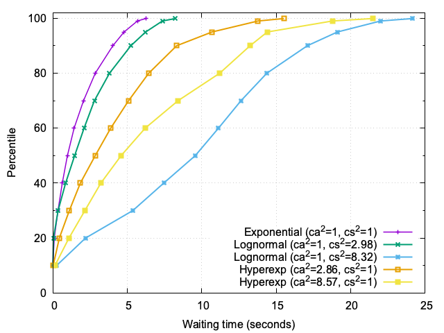
These results underscores a crucial observation: the impact of variability becomes more pronounced as system load increases. At 95% utilization, even small fluctuations in traffic or service times can lead to disproportionately long waiting times for some users. This highlights the importance of proactive measures to manage variability and maintain a consistent user experience.
2.1. Managing variability
Admission control: In this experiment, admission control was intentionally disabled to observe the full effects of variability. However, in other scenarios, we applied a threshold of 30 seconds for expected waiting time. In the case of a hard cap, jobs are strictly rejected once the expected waiting time exceeds 30 seconds. However, with the sigmoid-based approach, rejection starts earlier, even before the 30-second threshold, as it uses a probabilistic algorithm. This means some jobs are still allowed through, even when the estimated wait exceeds 30 seconds, ensuring a smoother and more gradual rejection process. For a detailed explanation of these algorithms, see Part 4.
Increasing capacity: Adding capacity is an effective way to mitigate variability, especially during peak loads. This can be achieved reactively, e.g., through autoscaling in cloud environments, or proactively, by forecasting demand and provisioning resources in advance. Both strategies help reduce the system’s sensitivity to traffic surges and service-time outliers.
Balancing load: Distributing traffic more evenly across servers or regions can also help manage variability. Techniques like load balancing ensure that no single server becomes a bottleneck, improving overall system resilience.
2.2. Operational insights
- Variability is not just a statistical artifact — it has real-world implications for user experience. Systems operating near capacity are particularly vulnerable to its effects.
- Admission control thresholds should be carefully calibrated based on tail metrics (e.g.,
p95orp99waiting times) rather than averages. This ensures that the system remains responsive even under high variability. - Capacity planning should account for both average load and variability. A system designed for 80% average utilization may still struggle if variability pushes peak loads beyond its limits.
By combining these strategies—sensible admission control, capacity scaling, and load balancing—systems can effectively manage variability and deliver a more predictable user experience, even under challenging conditions.
2.3. Queue size and traffic variability
To further explore the impact of variability on system performance, we conducted an experiment with bursty traffic (ca²=8) and heavy-tailed service times (cs²=8), while keeping the other parameters as described in Section 1.
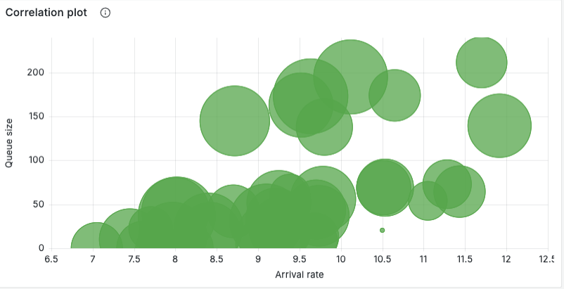
The results are visualized in a correlation plot (Figure 2), showing the relationship between instantaneous arrival rate (x axis) and observed queue size (y axis) for sampled intervals during the experiment; each point is a sample and the circle area encodes the average service time during that sample. Read this plot as a compact fingerprint of how demand and service interact:
- Diagonal trend: as arrival rate increases, queue size tends to grow — this is the expected load-driven behavior. The slope of the cloud gives a sense of how sensitively the queue reacts to additional load under current capacity and admission policy.
- Vertical spread at a given arrival rate: when points at similar x values show a wide range of y values, service-time variability is the likely cause — some intervals include long-running jobs (large circle sizes) that inflate the queue even when arrival rate is moderate.
- Large circles at moderate arrival rates are important: they show that long service times (or sudden processing slowdowns) can cause large backlogs without an increase in offered load. These are the scenarios where techniques such as job segregation (see Section 3.2), timeouts or specialized pools pay off.
These results highlight the complex interplay between arrival rates, queue sizes, and service times under high variability and sustained load. The clusters and outliers provide valuable insights into how variability manifests in real-world scenarios, emphasizing the need for robust strategies to manage such conditions effectively.
From an operational standpoint, this panel can be used to:
- Tune admission thresholds or parameters by observing the arrival-rate where queue size starts growing rapidly.
- Investigate large-circle samples to find slow jobs or degraded backend components.
- Use per-source coloring or faceting to detect noisy clients that produce disproportionate queue growth and consider per-source quotas for them.
📊 Measurement note
2.3.1. Analyzing waiting times: bursts vs. large jobs
To better understand the causes of queuing delays, we analyzed waiting times during the experiment described in Section 2.3. Specifically, we categorized large waits based on their root causes: bursts of arrivals or large service times. The results are visualized in Figure 3, which shows all waiting times over the 20-minute experiment as dots, along with additional annotations:
- Blue line: The average waiting time over every 50 jobs, providing a smoothed trend of overall system behavior.
- Green “X” markers: Highlighted waits caused by bursts of arrivals, identified as jobs with interarrival times in the fastest 5% (burst percentile).
- Red dots: Highlighted waits caused by large service times, identified as jobs with service times in the largest 5% (large service percentile).
- Threshold: Only waits above 5 seconds are highlighted to focus on significant delays.
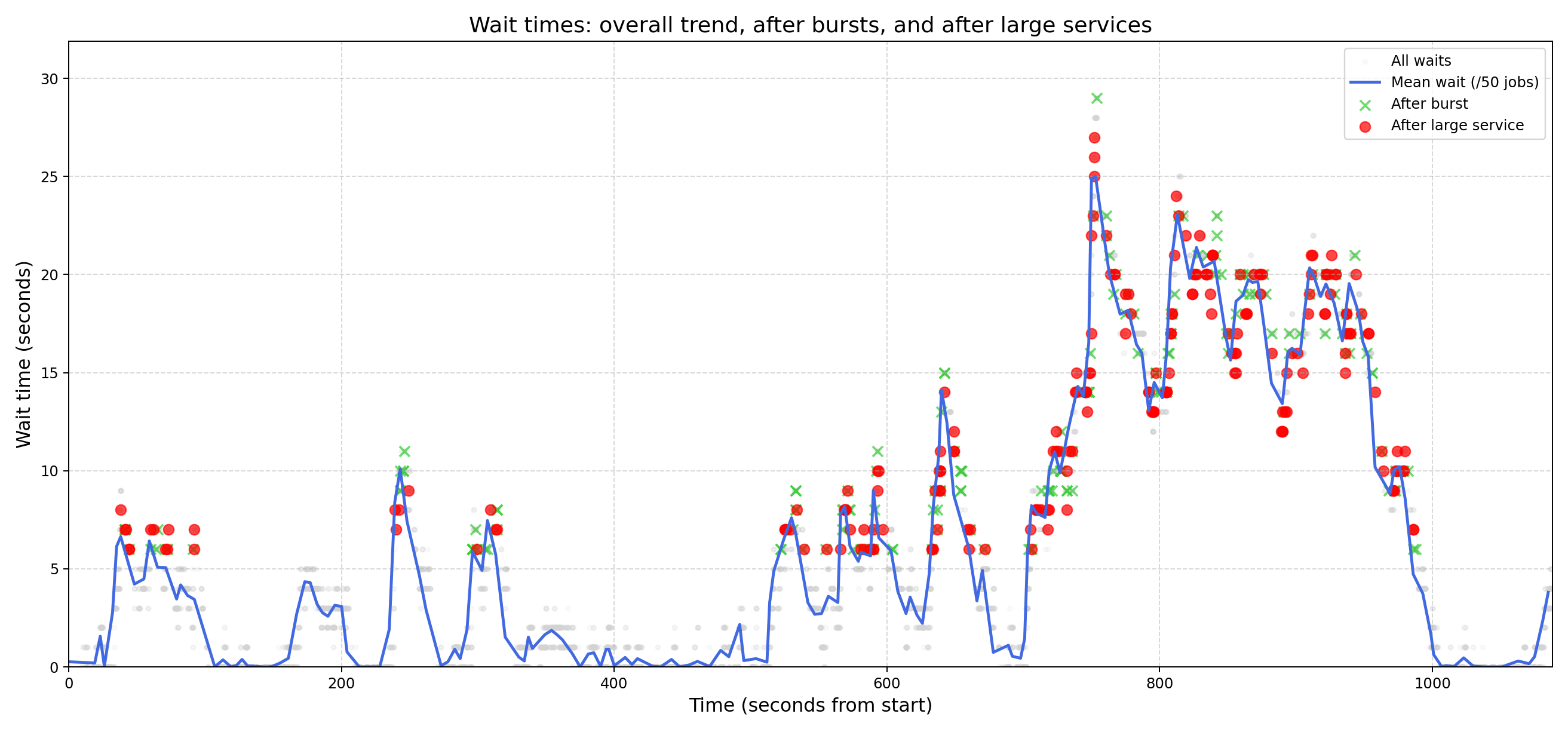
The chart shows significantly more “red dots” (large service times) than “green X” markers (bursts). This indicates that the system is better equipped to handle bursts of arrivals than large jobs. With 10 servers, bursts are naturally distributed across the pool, reducing their impact on any single queue. In contrast, large jobs monopolize server resources, effectively reducing capacity and causing prolonged delays.
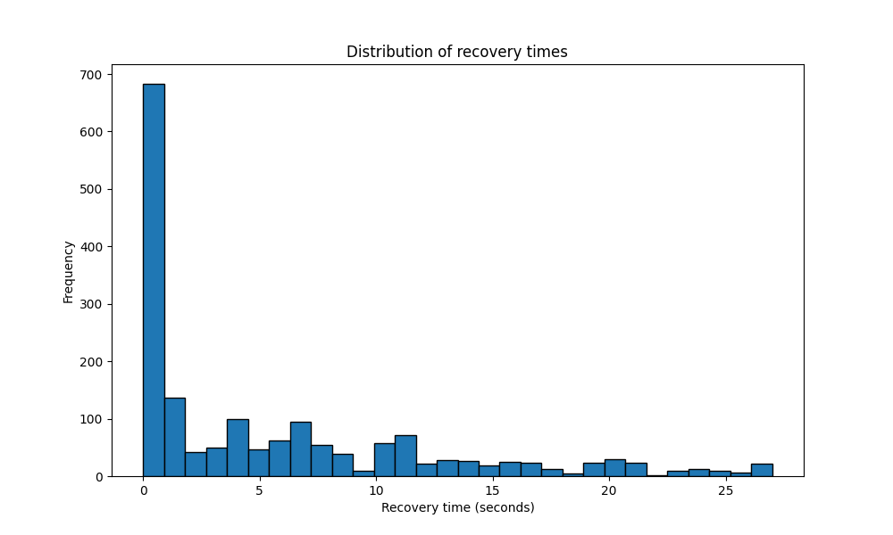
2.3.2. Recovery time distribution
To evaluate how quickly the system recovers from significant queuing events, we analyzed the distribution of recovery times during the experiment. Recovery time is defined as the duration it takes for the system to return to a steady state after a significant queuing event. The results are visualized in Figure 4, which shows the frequency of recovery times across the 20-minute experiment.
Definitions:
- Significant event: A queuing delay exceeding 1.5 times the 75th percentile of waiting times.
- Recovery: The time it takes for the system to return to the 90th percentile of waiting times.
Observations
- Fast recovery for most events: The majority of recovery times are within a couple of seconds, indicating that the system is generally resilient to transient spikes in queuing delays.
- Heavy-tailed distribution: While most recovery times are short, the distribution has a heavy tail, with some recovery times exceeding 25 seconds. These outliers correspond to periods of extreme variability, such as prolonged large jobs or overlapping bursts.
- High-percentile impact: The heavy tail in recovery times is a key factor driving high-percentile waiting time metrics (e.g., p95, p99). These prolonged recovery periods, while infrequent, have a disproportionate impact on user experience during peak load.
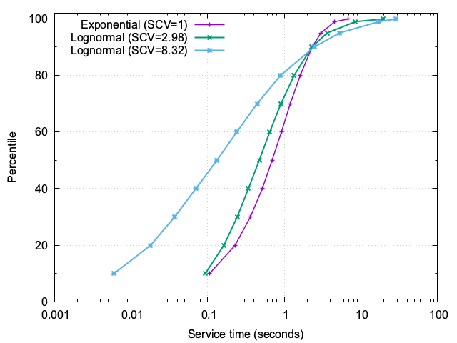
3. CDF of service times
Figure 5 illustrates the cumulative distribution of service times under three different levels of variability (cs²):
- cs² = 1: Exponential distribution, where service times are relatively consistent. Most jobs complete within a narrow range, with the 99th percentile at approximately 4.6 seconds.
- cs² = 2.98: Moderate variability introduces a noticeable spread. While the majority of jobs remain fast, the 99th percentile jumps to 8.5 seconds, and the 99.9th percentile reaches nearly 19.4 seconds.
- cs² = 8.32: Extreme variability creates a stark contrast. Many jobs are completed almost instantaneously, but a small fraction take disproportionately long, with the 99th percentile at 17.2 seconds and the 99.9th percentile exceeding 28 seconds.
3.1. Educational insights
When cs² is high, the service-time distribution becomes highly skewed. This means that while most jobs are very fast, a few outliers dominate the tail. These long jobs have a cascading effect on the system:
- Backlog formation: Long jobs monopolize server capacity, causing subsequent requests to queue up. This increases waiting times for all users, not just those directly affected by the long jobs. Here having several slow servers instead of a few fast one helps, as “small” jobs won’t get stuck behind a “large” one.
- Tail amplification: The presence of extreme outliers inflates high-percentile metrics (e.g.,
p95,p99), making the system appear less responsive overall. - Unpredictability: Users experience inconsistent performance, with some enjoying near-instantaneous service while others face significant delays.
3.2. Operational implications
- Job segregation: Separate long-running tasks from shorter ones to prevent them from blocking critical paths. This can be achieved through size-based routing or dedicated server pools. This paper discusses such technique in more details
- Timeouts and caps: Enforce timeouts or maximum job sizes to limit the impact of extreme outliers.
- Capacity planning: Design systems with sufficient headroom to absorb the effects of high service-time variability. This is especially important in scenarios where cs² is expected to escalate.
By understanding the dynamics of service-time variability, operators can implement targeted strategies to mitigate its impact, ensuring a more predictable and efficient system.
4. Queue-size histogram over time
The histogram of queue sizes shown in Figure 6 provides a clear visualization of how different traffic and service-time scenarios impact system behavior over a 20-minute trace. We compare three cases: (1) Markovian traffic, (2) bursty arrivals (ca²=8), and (3) black swan service times (cs²=8).
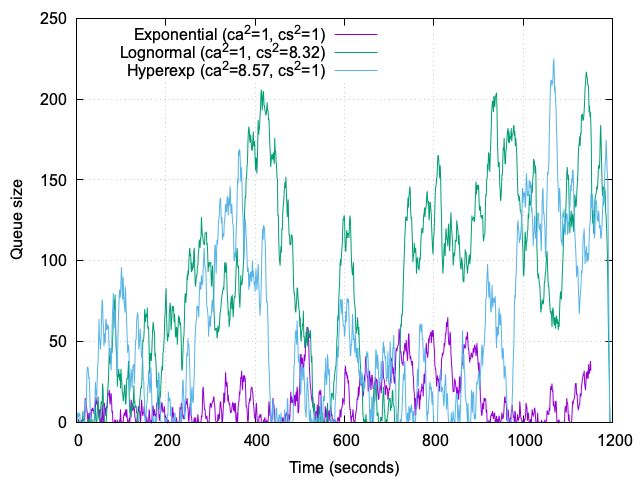
Markovian traffic: Under Markovian traffic, the system exhibits stability and predictability. The queue size frequently drops to zero, indicating idle periods, while the maximum queue size remains around 60. This reflects a well-balanced system operating near capacity without significant disruptions.
Bursty arrivals (ca²≈8): High interarrival variability introduces substantial congestion. The histogram reveals three major peaks where the queue size exceeds 200, interspersed with quieter periods. These peaks highlight the system’s difficulty in managing bursts, which can lead to temporary backlogs and degraded user experience.
Lognormal service times (cs²≈8): Heavy-tailed service times result in a different pattern. The histogram shows a single significant spike where the queue size exceeds 200, with prolonged periods (over 3 minutes) where the queue size remains above 100. This indicates that while the system can recover from isolated extreme events, the presence of heavy-tailed service times still introduces unpredictability and sustained large backlogs.
4.1. Comparison and insights
The comparison highlights the distinct challenges posed by each scenario:
- Markovian traffic: Predictable and stable, with minimal queuing issues.
- Bursty arrivals: Temporary congestion during bursts, requiring strategies like admission control or traffic shaping.
- Lognormal service times: Prolonged large backlogs, emphasizing the need for mechanisms to handle outliers, such as job segregation or timeouts.
These insights reinforce the importance of tailoring operational strategies to the specific variability characteristics of the traffic and service times.
5. Comparing 10-server and 100-server systems
To evaluate the impact of system size on performance under variability, we compared a 10-server system with a 100-server system, see Figure 7. Both systems were operated at 95% load, with ca²=1 (Markovian arrivals) and cs²=8 (heavy-tailed service times). The load was scaled proportionally to the number of servers to maintain consistent utilization.
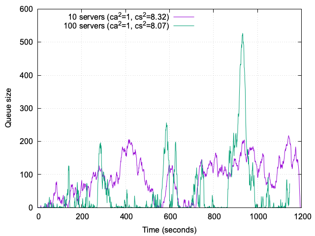
100-server system: The larger system demonstrates a remarkable ability to handle traffic variability. The histogram shows many quiet periods, with only a couple of short spikes where the queue size reaches 200 and one larger spike exceeding 500. However, even the largest spike corresponds to just 5 seconds of waiting time, thanks to the high server count. This highlights the system’s resilience and ability to quickly absorb variability without significant queuing.
10-server system: In contrast, the smaller system struggles more with variability. The histogram reveals long intervals where the queue size exceeds 100 and reaches up to 200 (corresponding to a waiting time of approximately 20 seconds), interspersed with some quiet periods. These prolonged backlogs indicate that the smaller system is less capable of absorbing the impact of black swan events, such as large jobs, rather than increased traffic. This leads to longer waiting times and reduced responsiveness.
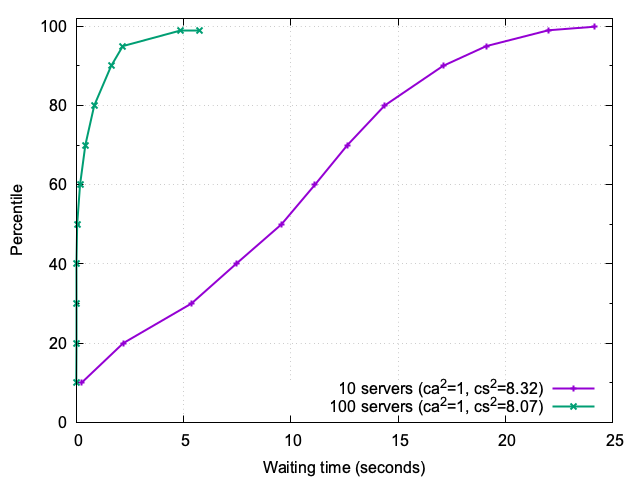
To further illustrate the differences between the 10-server and 100-server systems, we analyzed the cumulative distribution function (CDF) of waiting times for the same experiment (ca²=1, cs²≈8), see Figure 8:
10-server system: The waiting-time CDF for the 10-server system highlights the challenges of handling heavy-tailed service times with limited capacity. High percentiles, such as the 99th and 99.9th, show waiting times exceeding 22 seconds, reflecting the impact of black swan events.
100-server system: In contrast, the 100-server system demonstrates much shorter waiting times across all percentiles. Even at the 99.9th percentile, waiting times remain below 6 seconds, showcasing the system’s ability to handle variability effectively.
5.1. Insights
The comparison between 10-server and 100-server systems highlights the importance of system size in handling variability. Larger systems demonstrate resilience and shorter waiting times, even under heavy-tailed service times. This sets the stage for exploring how admission control strategies and client patience further influence system behavior.
6. Comparing admission control and client patience
This section explores the system’s behavior under varying traffic conditions, admission control strategies, and client patience levels. We analyze three scenarios: (1) light traffic, (2) saturated system, and (3) overloaded system, using both the hard cap and sigmoid-based admission control mechanisms we have described in our previous article. Additionally, we compare clients with finite patience to those with infinite patience.
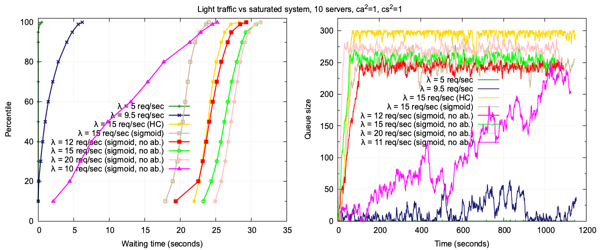
For this set of experiments, we go back to our default system (10 servers) and use Markovian traffic (ca²=1, cs²=1). Figure 9 provides several insights:
Light traffic (λ = 5): Under light traffic, the system operates at 50% load. The queue size remains at zero throughout the 20-minute trace, and waiting times are minimal:
- p95: 5 ms
- p99.9: 500 ms
This scenario demonstrates the system’s ability to handle low traffic efficiently, with negligible queuing and near-instantaneous response times.
Saturated system (λ = 9.5): At 95% load, the system exhibits periods of queue growth, reaching up to 60, interspersed with quiet periods. The
p95waiting time is not approximately 4.7 seconds, reflecting a well-utilized system that occasionally experiences moderate queuing but remains responsive overall.Overloaded system (λ = 15), Hard Cap admission control: In this scenario, the system is overloaded by 50% (capacity is 10 jobs per second). The hard cap admission control rejects jobs when the expected waiting time exceeds 30 seconds. The queue size grows rapidly and stabilizes at around 300 after 1 minute, corresponding to the 30-second waiting time cap. The waiting-time CDF is as follows:
- p95: 26.306 seconds
- p99.9: 28.317 seconds
This behavior highlights the hard cap’s ability to enforce a strict upper limit on waiting times, albeit at the cost of a large, stable queue.
Overloaded system (λ = 15), Sigmoid admission control: Replacing the hard cap with a sigmoid-based admission control results in a more aggressive rejection of jobs as the queue grows. The queue size stabilizes at around 250, lower than with the hard cap. The waiting-time CDF shows:
- p95: 22.756 seconds
- p99.9: 24.049 seconds
The sigmoid function smooths the admission control behavior, reducing both the queue size and waiting times compared to the hard cap, as it rejects some jobs even when the expected waiting time is smaller than the threshold.
6.1. Client patience
In the previous experiments clients had finite patience, with an average of 10 seconds. At each polling event, clients evaluated their estimated waiting time and abandoned the queue probabilistically.
This model captures the likelihood of abandonment as a function of the estimated waiting time and the client’s patience. However, it is important to note that no closed-form solution exists for this model. As a result, it is not possible to analytically estimate the average behavior of clients in terms of patience. This necessitates the use of simulation-based approaches to understand and predict client abandonment behavior under different conditions.
Next we analyze the system’s behavior when clients have infinite patience, never abandoning the queue.
6.2. Infinite patience and Sigmoid admission control
In this set of experiments, we assume clients have infinite patience and use sigmoid-based admission control. This configuration allows us to observe how the system behaves under varying levels of traffic, from saturation to extreme overload.
λ = 10 (saturated system): At 100% capacity, the system is saturated. The queue grows slowly but unbounded, with occasional periods of shrinkage. By the end of the 20-minute experiment, the queue size exceeds 200. If the experiment were extended to 1 hour, the queue would likely reach the point where the sigmoid admission control takes over more aggressively. The waiting-time CDF is as follows:
- p50: 9.805 seconds
- p95: 22.924 seconds
- p99.9: 25.215 seconds
λ = 12 (20% overloaded): With a 20% overload, the queue grows quickly but stabilizes at around 240. The sigmoid admission control ensures that a fraction of traffic continues to flow through the system, even as the arrival rate increases. This behavior results in a smaller queue size compared to higher arrival rates. The waiting-time CDF is as follows:
- p50: 24.120 seconds
- p95: 27.229 seconds
- p99.9: 29.319 seconds
λ = 15 (50% overloaded): At 50% overload, the queue size is higher than in scenarios where clients may abandon the system. Infinite patience leads to prolonged queuing, as no clients leave the system regardless of wait times. The waiting-time CDF is as follows:
- p50: 26.237 seconds
- p95: 29.254 seconds
- p99.9: 31.342 seconds
λ = 20 (100% overloaded): At double the system’s capacity, the queue grows rapidly to about 280. Interestingly, while the queue size is smaller than in the hard cap admission control scenario with λ = 15, the waiting-time CDF is worse. This is because clients never abandon the system, even when waiting times are extremely long. The waiting-time CDF is as follows:
- p50: 27.168 seconds
- p95: 29.654 seconds
- p99.9: 31.343 seconds
These experiments highlight the impact of infinite patience on system performance. While sigmoid admission control helps manage queue sizes, the absence of client abandonment leads to longer waiting times, particularly under extreme overload conditions. This underscores the importance of considering client behavior when designing admission control strategies.
⏳ Similarity in higher percentiles
7. Extreme overload: edge shedding and server admission (≈60× peak load)
We ran a targeted experiment to exercise the edge “gate” (OpenResty) and the server-side sigmoid admission control under Markovian traffic (ca²=1, cs²=1). As before, the system capacity is 10 requests/second (10 servers and average service time of 1 second):
- Baseline load: 15 req/sec (the setup is running under a sustained overload relative to service capacity; admission control is active on the server and returns HTTP 429 for rejected requests)
- Spike pattern: as shown in Figure 6, every few minutes a second client is started; for 2 minutes each time it generates bursts of 300, 400, 500 and 600 req/sec (one burst per level)
- Sigmoid based admission control on the server, with threshold set to 30 seconds
- Clients patience as discussed in Section 6.1.
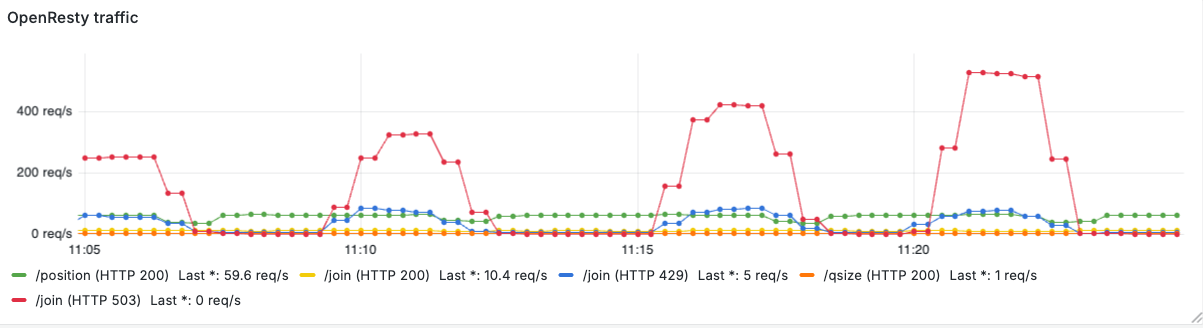
This test is intentionally designed to stress the system’s double-layer admission control. Please note that the peak offered load in the largest burst reaches roughly 615 req/sec (baseline 15 plus 600), which corresponds to over 60× the system capacity (10 req/sec). The goal is to observe how edge shedding and server-side admission interact under extreme, transient overloads, including any overshoot caused by sampling and control-loop delays.
What we observed
As shown in Figure 10, the edge gate drops the majority of the extra traffic with HTTP 503. Measured drop counts for the injected bursts were approximately:
- During the first burst (extra 300 req/sec), 250 req/sec got dropped at the edge
- During the second burst (extra 400 req/sec), about 320 req/sec got dropped at the edge
- During the third traffic spike (extra 500 req/sec) our gate rejected about 420 req/sec
- In the final burst (extra 600 req/sec), OpenResty dropped approximately 525 req/sec
Figure 11 shows how the residual excess traffic that makes it past the gate is handled by the server’s admission control: the rejected line indicates the rate at which the backend drops traffic (HTTP 429), while join reports the rate of requests that enter the queue. As you can see, it matches the processed value, indicating the system was saturated.
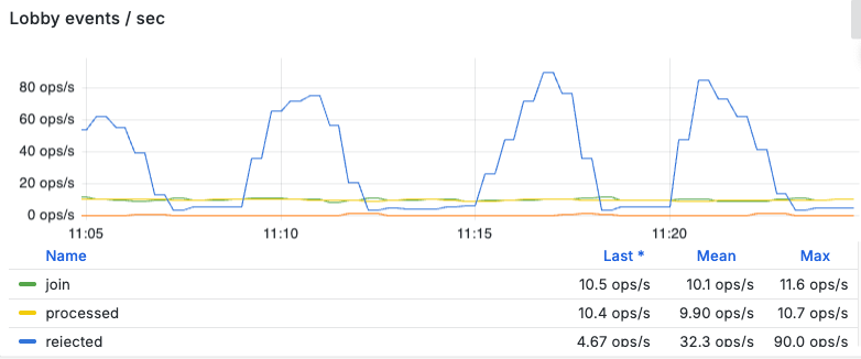
Queue and latency behavior
Figure 12 shows that during the large spikes the server-side queue grows to about 330 queued requests (peak observed during the highest bursts) - with values being sampled once per second.
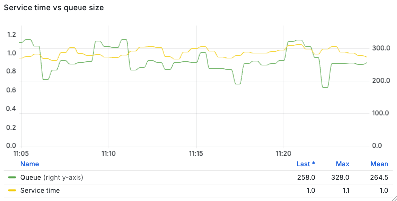
Why ≈330 (corresponding to waiting time of approximately 33 seconds, since the system can handle only an average of 10 jobs/sec)? The gate admits a small fraction of the offered load, and that admitted traffic accumulates at the backend while the service capacity is fixed. Thus, the queue increases until the effective admission probability produced by the sigmoid controller balances service throughput.
Short, sharp spikes can overshoot this balance because the gate reads the controller state from Redis only once per second — so a sudden surge during the test can send over 500 requests past the gate in the interval before the OpenResty tightens its drop rate.
As a reminder: the edge gate polls a Redis key (written by the lobby’s elected leader) once per second to fetch the current reject probability. That value is used by hysteresis at the gate to avoid flapping, with Redis being the source of truth for the admission-control state.
In spite of the backlog, the observed waiting-time statistics (server queue) during the bursts were:
- Average waiting time: 26.75 s
p95: 32.5 sp99: 34.9 s
Finally, customer-facing endpoints (/join, /position, /qsize) remain fast because they are lightweight lookups and do not wait for the expensive backend processing. Measured p99 latency for these endpoints during bursts is 4 ms — see the latency panel in Figure 13 below.
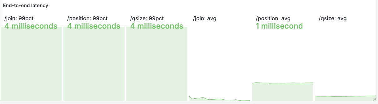
p99 and average) for /join, /position, /qsize recorded during the experiment. These endpoints are served quickly because they avoid expensive backend work.8. Practical insights for designing Lobby systems
Admission control strategy: Use adaptive admission control mechanisms like sigmoid functions or leaky bucket to dynamically manage traffic. These mechanisms ensure that some traffic always flows through the system, preventing complete gridlock while maintaining fairness.
Client patience modeling: Understand the patience behavior of your clients. Infinite patience, while useful for theoretical analysis, is rarely realistic. Incorporating probabilistic abandonment models can help you design systems that better reflect real-world behavior and reduce extreme waiting times.
Queue size management: Monitor and manage queue sizes proactively. Overload conditions can lead to unbounded queue growth, which may not only degrade user experience, but also affect system stability. Implementing thresholds or alerts for queue size can help operators intervene when necessary.
Waiting-time distribution: Pay attention to the entire waiting-time distribution, not just averages. High percentiles (e.g., p90, p95) often reveal the worst-case scenarios that users may experience, which are critical for system design and user satisfaction.
Scalability and elasticity: Design the system to scale elastically under high load. This could involve spinning up additional resources or redirecting traffic to alternative queues or systems during peak times.
Feedback loops: Provide real-time feedback to users about their estimated wait times. Transparency can improve user satisfaction and reduce frustration, even in overload conditions.
Stress testing: Simulate overload scenarios during testing to understand how the system behaves under extreme conditions. This helps identify bottlenecks and ensures the system can recover gracefully.
Prioritization mechanisms: Consider implementing prioritization for certain types of users or requests. For example, premium users or critical requests could be given higher priority in the queue, and certain paths (e.g.,
/position) dedicated resources.
Conclusions
The performance evaluation we have conducted in this article surfaces a few simple, operational truths that should guide any lobby design:
- Admission control is essential. A smooth controller (sigmoid) reduces shock, but it should be paired with a strict cap to avoid unbounded queues under extreme load.
- Model client behavior. Infinite-patience assumptions amplify tails, while realistic abandonment models materially change optimal policies and tail risk.
- Size matters. Queueing theory tells us that larger pools absorb variability far better than small pools - and the experiments we have discussed in this article confirmed it; when possible, prefer scale (or elastic capacity) to brittle tight provisioning.
- Variability dominates averages. Tail metrics (
p95/p99/p99.9) should be your primary SLO signals — tune controls against them, not the mean. - Defense in depth works. Edge shedding (OpenResty gate) plus server-side admission gives predictable degradation and preserves lightweight endpoints.
- Invest in observability. Track admitted vs dropped (edge 503 vs server 429), queue size, and tail waiting times at high resolution (e.g., 1 second); correlate metrics such as queue size with service-time outliers and per-source activity. While our proof-of-concept uses simple metrics, advanced tools like eBPF and OpenTelemetry can significantly enhance visibility and simplify root cause analysis, especially in distributed systems where requests traverse multiple services.
By incorporating these insights, developers and system architects can build lobby systems that not only handle overload conditions effectively but also provide a better user experience.
💡 A note on reproducibility and source
📬 Get weekly queue insights
Not ready to talk? Stay in the loop with our weekly newsletter — The Queue Report, covering intelligent queue management, digital flow, and operational optimization.